Programmable Filter Coefficients for FIR Filters
Note
The Filter Design HDL Coder™ product will be discontinued in a future release. Instead, you can model hardware behavior, and generate HDL code by using System objects or Simulink® blocks from DSP HDL Toolbox™. These objects and blocks include hardware-friendly control signals and architecture options. To generate HDL code from DSP HDL Toolbox objects and blocks, you must also have the HDL Coder™ product.
For examples of modeling a programmable FIR filter for hardware, see Programmable FIR Filter for FPGA and Optimize Programmable FIR Filter Resources (DSP HDL Toolbox). These examples use the
Discrete FIR Filter (DSP HDL Toolbox) block. Equivalent functionality is also available in the
dsphdl.FIRFilter (DSP HDL Toolbox)
System object™.
By default, the coder obtains filter coefficients from a filter object and hard-codes them into the generated code. An HDL filter realization generated in this way cannot be used with a different set of coefficients.
For direct form FIR filters, the coder provides UI options and corresponding command-line properties that let you:
Generate an interface for loading coefficients from memory. Coefficients stored in memory are called programmable coefficients.
Test the interface.
Programmable filter coefficients are supported for these direct form FIR filter types:
Direct form
Direct form symmetric
Direct form antisymmetric
To use programmable coefficients, a port interface (referred to as a processor interface) is generated for the filter entity or module. Coefficient loading is assumed to be under the control of a microprocessor that is external to the generated filter. The filter uses the loaded coefficients for processing input samples.
Programmable filter coefficients are supported for these filter architectures:
Fully parallelFully serialPartly serialCascade serial
When you choose a serial FIR filter architecture, you can also specify how the coefficients are stored. You can select a dual-port or single-port RAM, or a register file. See Programmable Filter Coefficients for FIR Filters.
You can also generate a processor interface for loading IIR filter coefficients. See Programmable Filter Coefficients for IIR Filters.
UI Options for Programmable Coefficients
These UI options let you specify programmable coefficients.
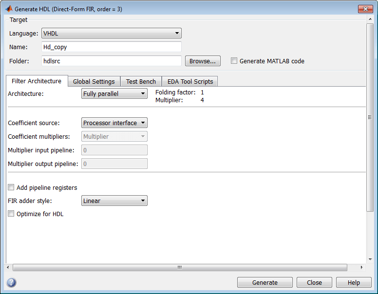
The Coefficient source list on the Generate HDL tool lets you select whether coefficients are obtained from the filter object and hard-coded (
Internal), or from memory (Processor interface). The default isInternal.The corresponding command-line property is
CoefficientSource.
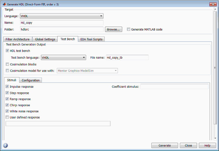
The Coefficient stimulus option on the Test Bench pane of the Generate HDL tool specifies how the test bench tests the generated memory interface.
The corresponding command-line property is
TestBenchCoeffStimulus.
Generating a Test Bench for Programmable FIR Coefficients
This section describes how to use the TestBenchCoeffStimulus property to specify how the test bench drives the
coefficient ports. You can also use the Coefficient stimulus option for
this purpose.
When a coefficient memory interface has been generated for a filter, the coefficient
ports have associated test vectors. The TestbenchCoeffStimulus property
determines how the test bench drives the coefficient ports.
The TestBenchStimulus
property determines the filter input stimuli.
The TestbenchCoeffStimulus property selects from two types of test
benches. TestbenchCoeffStimulus takes a vector argument. The valid values
are:
[]: Empty vector. (default)When the value of
TestbenchCoeffStimulusis an empty vector, the test bench loads the coefficients from the filter object, and then forces the input stimuli. This test verifies that the interface writes one set of coefficients into the memory without encountering an error.[
coeff1,coeff2,...coeffN]: Vector ofNcoefficients, whereNis determined as follows:For symmetric filters,
Nmust equalceil(length(filterObj.Numerator)/2).For antisymmetric filters,
Nmust equalfloor(length(filterObj.Numerator)/2).For other filters,
Nmust equal the length of the filter object.
In this case, the filter processes the input stimuli twice. First, the test bench loads the coefficients from the filter object and forces the input stimuli to show the response. Then, the filter loads the set of coefficients specified in the
TestbenchCoeffStimulusvector, and shows the response by processing the same input stimuli for a second time. In this case, the internal states of the filter, as set by the first run of the input stimulus, are retained. The test bench verifies that the interface writes two different sets of coefficients into the coefficient memory. The test bench also provides an example of how the memory interface can be used to program the filter with different sets of coefficients.
Note
If a coefficient memory interface has not been previously generated for the filter,
the TestbenchCoeffStimulus property is ignored.
For an example, see .
Using Programmable Coefficients with Serial FIR Filter Architectures
This section discusses special considerations for using programmable filter coefficients with FIR filters that have one of these serial architectures.
Fully serialPartly serialCascade serial
Specifying Memory for Programmable Coefficients
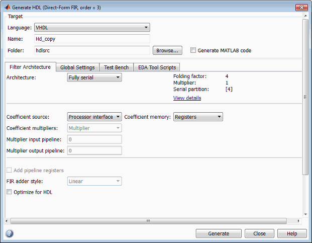
By default, the processor interface for programmable coefficients loads the coefficients from a register file. The Coefficient memory pull-down menu lets you specify alternative RAM-based storage for programmable coefficients.
You can set Coefficient memory when:
The filter is a FIR filter.
You set Coefficient source to
Processor interface.You set Architecture to
Fully serial,Partly serial, orCascade serial.
The figure shows the Coefficient memory option for a fully serial FIR filter. You can select an option using the drop-down list.

The table summarizes the Coefficient memory options.
| Coefficient memory Selection | Description |
|---|---|
Registers | default: Store programmable coefficients in a register file. |
Single Port RAMs | Store programmable coefficients in single-port RAM. The coder writes each RAM and its interface to a separate file. The number of generated RAMs depends on the filter partitioning. |
Dual Port RAMs | Store programmable coefficients in dual-port RAM. The coder writes each RAM and its interface to a separate file. The number of generated RAMs depends on the filter partitioning. |
Timing Considerations
In a serial implementation of a FIR filter, the rate of the system clock
(clk) is generally a multiple of the input data rate (the sample rate
of the filter). The exact relationship between the clock rate and the data rate depends on
your choice of serial architecture and partitioning options.
Programmable coefficients load into the coeffs_in port at either
the system clock rate (faster) or the input data (slower) rate. If your design requires
loading of coefficients at the faster rate, observe these points.
When
write_enableasserts, coefficients load from thecoeffs_inport into coefficient memory at the address specified bywrite_address.write_donecan assert for anynumber of clock cycles. Ifwrite_doneasserts at least twoclkcycles before the arrival of the next data input value, new coefficients will be applied with the next data sample. Otherwise, new coefficients will be applied for the data after the next sample.
These two examples illustrate how serial partitioning affects the timing of coefficient loading.
Create a direct form filter with 11 coefficients.
rng(13893,'v5uniform');
b = rand(1,11);
filt = dsp.FIRFilter('Numerator',b,'Structure','Direct form');
Generate VHDL® code for filt, using a partly serial architecture with
the serial partition [7 4]. Set CoefficientSource to
generate a processor interface.
generatehdl(filt,'InputDataType',numerictype(1,16,15), ...
    'SerialPartition',[7 4],'CoefficientSource','ProcessorInterface');
### Clock rate is 7 times the input sample rate for this architecture.
### HDL latency is 3 samples
This partitioning results in a clock rate that is seven times the input sample rate.
The timing diagram illustrates the rate of coefficient loading relative to the rate of
input data samples. While write_enable is asserted, 11 coefficient
values are loaded, via coeffs_in, to 11 sequential memory addresses. On
the next clk cycle, write_enable is deasserted and
write_done is asserted for one clock period. The coefficient loading
operation is completed within two cycles of data input, allowing 2 clk
cycles to elapse before the arrival of the data value 07FFF. Therefore
the newly loaded coefficients are applied to that data sample.

Now define a serial partition of [6 5] for the same filter. This
partition results in a slower clock rate, six times the input sample rate.
generatehdl(filt,'InputDataType',numerictype(1,16,15), ...
    'SerialPartition',[6 5],'CoefficientSource','ProcessorInterface');
### Clock rate is 6 times the input sample rate for this architecture.
### HDL latency is 3 samples
The timing diagram illustrates that write_done deasserts too late
for the coefficients to be applied to the arriving data value 278E.
They are applied instead to the next sample, 7FFF.

