Effects of Multiobjective Genetic Algorithm Options
This example shows some of the effects of multiobjective genetic algorithm options. You create and change options for gamultiobj using the optimoptions function.
Setting Up a Problem for gamultiobj
gamultiobj finds a local Pareto front for multiple objective functions using the genetic algorithm. For this example, use gamultiobj to obtain a Pareto front for two objective functions described in the function kur_multiobjective.m. This represents a real-valued function that consists of two objectives, each of three decision variables. Also impose bound constraints on the decision variables -5 <= x(i) <= 5, i = 1,2,3.
function y = kur_multiobjective(x)
%KUR_MULTIOBJECTIVE Objective function for a multiobjective problem.
%   The Pareto-optimal set for this two-objective problem is nonconvex as
%   well as disconnected. The function KUR_MULTIOBJECTIVE computes two
%   objectives and returns a vector y of size 2-by-1.
%
%   Reference: Kalyanmoy Deb, "Multi-Objective Optimization using
%   Evolutionary Algorithms", John Wiley & Sons ISBN 047187339

%   Copyright 2007 The MathWorks, Inc.


% Initialize for two objectives
y = zeros(2,1);

% Compute first objective
for i = 1:2
  y(1) = y(1)  - 10*exp(-0.2*sqrt(x(i)^2 + x(i+1)^2));
end

% Compute second objective
for i = 1:3
   y(2) = y(2) +  abs(x(i))^0.8 + 5*sin(x(i)^3);
end
end
To observe the solver progress, plot the Pareto front in every generation using the plot function @gaplotpareto. Specify this plot function in the options by using the optimoptions function.
FitnessFunction = @kur_multiobjective; % Function handle to the fitness function
numberOfVariables = 3; % Number of decision variables
lb = [-5 -5 -5]; % Lower bound
ub = [5 5 5]; % Upper bound
A = []; % No linear inequality constraints
b = []; % No linear inequality constraints
Aeq = []; % No linear equality constraints
beq = []; % No linear equality constraints
options = optimoptions(@gamultiobj,PlotFcn=@gaplotpareto);
Run the gamultiobj solver and display the number of solutions found on the Pareto front and the number of generations.
[x,Fval,exitFlag,Output] = gamultiobj(FitnessFunction,numberOfVariables,A, ...
    b,Aeq,beq,lb,ub,options);
gamultiobj stopped because the average change in the spread of Pareto solutions is less than options.FunctionTolerance.
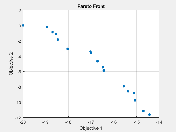
fprintf("The number of points on the Pareto front was: %d\n", size(x,1));The number of points on the Pareto front was: 18
fprintf("The number of generations was : %d\n", Output.generations);The number of generations was : 317
The Pareto plot displays two competing objectives. For this problem, the Pareto front is known to be disconnected. The solution from gamultiobj can capture the Pareto front even if it is disconnected. Note that when you run this example, your result may be different from the results shown because gamultiobj uses random number generators.
Elitist Multiobjective Genetic Algorithm
The multiobjective genetic algorithm (gamultiobj) works on a population using a set of operators that are applied to the population. A population is a set of points in the design space. The initial population is generated randomly by default. The next generation of the population is computed using the non-dominated rank and a distance measure of the individuals in the current generation.
A non-dominated rank is assigned to each individual using the relative fitness. Individual 'p' dominates 'q' ('p' has a lower rank than 'q') if 'p' is strictly better than 'q' in at least one objective and 'p' is no worse than 'q' in all objectives. This is the same as saying 'q' is dominated by 'p' or 'p' is non-inferior to 'q'. Two individuals 'p' and 'q' are considered to have equal ranks if neither dominates the other. The distance measure of an individual is used to compare individuals with equal rank. It is a measure of how far an individual is from the other individuals with the same rank.
The multiobjective GA function gamultiobj uses a controlled elitist genetic algorithm (a variant of NSGA-II [1]). An elitist GA always favors individuals with better fitness value (rank) whereas, a controlled elitist GA also favors individuals that can help increase the diversity of the population even if they have a lower fitness value. It is very important to maintain the diversity of population for convergence to an optimal Pareto front. This is done by controlling the elite members of the population as the algorithm progresses. Two options ParetoFraction and DistanceFcn are used to control the elitism. The Pareto fraction option limits the number of individuals on the Pareto front (elite members) and the distance function helps to maintain diversity on a front by favoring individuals that are relatively far away on the front.
Specifying Multiobjective GA Options
We can chose the default distance measure function, distancecrowding, that is provided in the toolbox or write our own function to calculate the distance measure of an individual. The crowding distance measure function in the toolbox takes an optional argument to calculate distance either in function space (phenotype) or design space (genotype). If "genotype" is chosen, then the diversity on a Pareto front is based on the design space. The default choice is "phenotype" and, in that case, the diversity is based on the function space. Here we choose "genotype" for our distance function. We will directly modify the value of the parameter DistanceMeasureFcn.
options.DistanceMeasureFcn = {@distancecrowding,"genotype"};The Pareto fraction has a default value of 0.35 i.e., the solver will try to limit the number of individuals in the current population that are on the Pareto front to 35 percent of the population size. Here we set the Pareto fraction to 0.5.
options = optimoptions(options,ParetoFraction=0.5);
Run the gamultiobj solver and display the number of solutions found on the Pareto front and the average distance measure of solutions.
[x,Fval,exitFlag,Output] = gamultiobj(FitnessFunction,numberOfVariables,A, ...
                                        b,Aeq,beq,lb,ub,options);
gamultiobj stopped because the average change in the spread of Pareto solutions is less than options.FunctionTolerance.

fprintf("The number of points on the Pareto front was: %d\n", size(x,1));The number of points on the Pareto front was: 25
fprintf("The average distance measure of the solutions on the Pareto front was: %g\n", Output.averagedistance);The average distance measure of the solutions on the Pareto front was: 0.051005
fprintf("The spread measure of the Pareto front was: %g\n", Output.spread);The spread measure of the Pareto front was: 0.181192
A smaller average distance measure indicates that the solutions on the Pareto front are evenly distributed. However, if the Pareto front is disconnected, then the distance measure will not indicate the true spread of solutions.
Modifying the Stopping Criteria
gamultiobj uses three different criteria to determine when to stop the solver. The solver stops when any one of the stopping criteria is met. It stops when the maximum number of generations is reached; by default this number is '200*numberOfVariables'. gamultiobj also stops if the average change in the spread of the Pareto front over the MaxStallGenerations generations (default is 100) is less than the tolerance specified in options.FunctionTolerance. The third criterion is the maximum time limit in seconds (default is Inf). Here we modify the stopping criteria to change the FunctionTolerance from 1e-4 to 1e-3 and increase MaxStallGenerations to 150.
options = optimoptions(options,FunctionTolerance=1e-3,MaxStallGenerations=150);
Run the gamultiobj solver and display the number of solutions found on the Pareto front and the number of generations.
[x,Fval,exitFlag,Output] = gamultiobj(FitnessFunction,numberOfVariables,A, ...
    b,Aeq,beq,lb,ub,options);
gamultiobj stopped because the average change in the spread of Pareto solutions is less than options.FunctionTolerance.
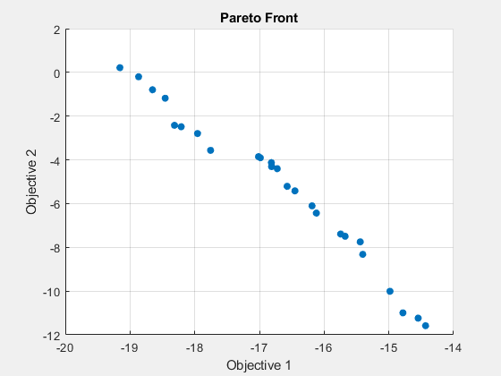
fprintf("The number of points on the Pareto front was: %d\n", size(x,1));The number of points on the Pareto front was: 25
fprintf("The number of generations was : %d\n", Output.generations);The number of generations was : 152
Multiobjective GA Hybrid Function
We will use a hybrid scheme to find an optimal Pareto front for our multiobjective problem. gamultiobj can reach the region near an optimal Pareto front relatively quickly, but it can take many function evaluations to achieve convergence. A commonly used technique is to run gamultiobj for a small number of generations to get near an optimum front. Then the solution from gamultiobj is used as an initial point for another optimization solver that is faster and more efficient for a local search. We use fgoalattain as the hybrid solver with gamultiobj. fgoalattain solves the goal attainment problem, which is one formulation for minimizing a multiobjective optimization problem.
The hybrid functionality in multiobjective function gamultiobj is slightly different from that of the single objective function GA. In single objective GA the hybrid function starts at the best point returned by GA. However, in gamultiobj the hybrid solver will start at all the points on the Pareto front returned by gamultiobj. The new individuals returned by the hybrid solver are combined with the existing population and a new Pareto front is obtained. It may be useful to see the syntax of fgoalattain function to better understand how the output from gamultiobj is internally converted to the input of fgoalattain function. gamultiobj estimates the pseudo weights (required input for fgoalattain) for each point on the Pareto front and runs the hybrid solver starting from each point on the Pareto front. Another required input, goal, is a vector specifying the goal for each objective. gamultiobj provides this input as the extreme points from the Pareto front found so far.
Here we run gamultiobj without the hybrid function.
[x,Fval,exitFlag,Output] = gamultiobj(FitnessFunction,numberOfVariables,A, ...
    b,Aeq,beq,lb,ub,options);
gamultiobj stopped because the average change in the spread of Pareto solutions is less than options.FunctionTolerance.
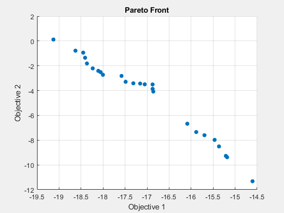
fprintf("The number of points on the Pareto front was: %d\n", size(x,1));The number of points on the Pareto front was: 25
fprintf("The average distance measure of the solutions on the Pareto front was: %g\n", Output.averagedistance);The average distance measure of the solutions on the Pareto front was: 0.0434477
fprintf("The spread measure of the Pareto front was: %g\n", Output.spread);The spread measure of the Pareto front was: 0.17833
Here we use fgoalattain as the hybrid function. We also reset the random number generators so that we can compare the results with the previous run (without the hybrid function).
options = optimoptions(options,HybridFcn=@fgoalattain);
Reset the random state (only to compare with previous run)
strm = RandStream.getGlobalStream;
strm.State = Output.rngstate.State;
Run the GAMULTIOBJ solver with hybrid function.
[x,Fval,exitFlag,Output,Population,Score] = gamultiobj(FitnessFunction,numberOfVariables,A, ...
    b,Aeq,beq,lb,ub,options);
gamultiobj stopped because the average change in the spread of Pareto solutions is less than options.FunctionTolerance.
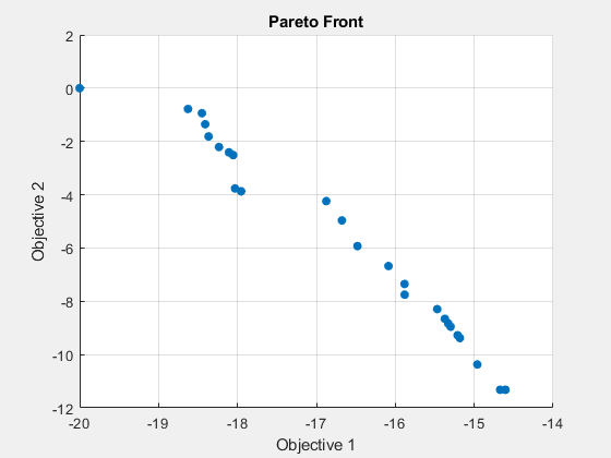
fprintf("The number of points on the Pareto front was: %d\n", size(x,1));The number of points on the Pareto front was: 25
fprintf("The average distance measure of the solutions on the Pareto front was: %g\n", Output.averagedistance);The average distance measure of the solutions on the Pareto front was: 0.128285
fprintf("The spread measure of the Pareto front was: %g\n", Output.spread);The spread measure of the Pareto front was: 0.420896
If the Pareto fronts obtained by gamultiobj alone and by using the hybrid function are close, we can compare them using the spread and the average distance measures. The average distance of the solutions on the Pareto front can be improved by using a hybrid function. The spread is a measure of the change in two fronts and that can be higher when hybrid function is used. This indicates that the front has changed considerably from that obtained by gamultiobj with no hybrid function.
It is certain that using the hybrid function will result in an optimal Pareto front but we may lose the diversity of the solution (because fgoalattain does not try to preserve the diversity). This can be indicated by a higher value of the average distance measure and the spread of the front. We can further improve the average distance measure of the solutions and the spread of the Pareto front by running gamultiobj again with the final population returned in the last run. Here, we should remove the hybrid function.
options = optimoptions(options,HybridFcn=[]); % No hybrid function
% Provide initial population and scores
options = optimoptions(options,InitialPopulationMatrix=Population,InitialScoresMatrix=Score);
% Run the GAMULTIOBJ solver with hybrid function.
[x,Fval,exitFlag,Output,Population,Score] = gamultiobj(FitnessFunction,numberOfVariables,A, ...
    b,Aeq,beq,lb,ub,options);
gamultiobj stopped because the average change in the spread of Pareto solutions is less than options.FunctionTolerance.
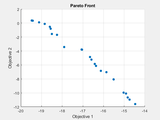
fprintf("The number of points on the Pareto front was: %d\n", size(x,1));The number of points on the Pareto front was: 25
fprintf("The average distance measure of the solutions on the Pareto front was: %g\n", Output.averagedistance);The average distance measure of the solutions on the Pareto front was: 0.0479902
fprintf("The spread measure of the Pareto front was: %g\n", Output.spread);The spread measure of the Pareto front was: 0.182761
References
[1] Kalyanmoy Deb, "Multi-Objective Optimization using Evolutionary
Algorithms", John Wiley & Sons ISBN 047187339.