Implement Hardware-Efficient Jacobi SVD for Two-by-Two Matrices
This example shows how to implement a hardware-efficient singular value decomposition (SVD) for real and complex two-by-two matrices, optimized for HDL applications.
The Square Jacobi SVD HDL Optimized block uses the two-sided Jacobi algorithm to compute the SVD for square matrices. This algorithm has inherent parallelism and performs well for FPGA and ASIC applications. The algorithm is iterative for a given n-by-n matrix. For the case of a real two-by-two matrix, this algorithm has a closed-form solution that can be implemented without iteration [1].
Real Two-by-Two Jacobi SVD Algorithm
If the input is a real two-by-two matrix
,
then the SVD of this matrix can be described as
where and .
The rotation angle and can be computed as follows:
Note that both and the matrix rotation can be efficiently computed by the CORDIC algorithm on hardware.
Complex Two-by-Two Jacobi SVD Algorithm
If the input matrix is a complex two-by-two matrix, then you can perform bidiagonalization to transform it into a real matrix first by following these CORDIC rotation steps [2]. In these equations, represents complex numbers, and represents real numbers such that the initial value of the , , and matrices can be represented as
, , and .
1. Rotate to real and apply the rotation to row 1 and .
is transformed into , where ,.
.
2. Rotate to real and apply the rotation to row 2 and such that
, where and .
.
3. Rotate rows 1 and 2 together to rotate to 0. Apply the same rotation to .
, where and .
.
4. Rotate to real and apply the rotation to column 2 and .
, where and .
.
5. Rotate to real and apply the rotation to .
, where and .
.
is now a real matrix. Continue with the real two-by-two SVD such that
,
, and
.
Implement Two-by-Two Jacobi SVD in MATLAB
The twoByTwoJacobiSVD function implements the algorithm described in the previous section for both two-by-two real and complex inputs. The twoByTwoJacobiSVD function is a special case of the fixed.jacobiSVD function.
Specify Simulation Parameters
Specify the dimension of the inputs, the number of input sample matrices, the input complexity, and word length.
n = 2;
numSamples = 3;
complexity = "complex";
wordLength = 16;
"complex";
wordLength = 16;Generate Input A Matrices
Use the specified simulation parameters to generate the input matrix A.
rng('default');
switch complexity
    case 'real'
        A = randn(n,n,numSamples);
    case 'complex'
        A = complex(randn(n,n,numSamples),randn(n,n,numSamples));
    otherwise
        A = randn(n,n,numSamples);
end
Compute Fixed-Point Data Types
Use the upper bound on the singular values to define fixed-point types that will never overflow. First, use the fixed.singularValueUpperBound function to determine the upper bound on the singular values.
svdUpperBound = fixed.singularValueUpperBound(n,n,max(abs(A(:))));
Define the integer length based on the value of the upper bound, with one additional bit for the sign, one additional bit for intermediate CORDIC growth, and one more bit for intermediate growth to compute the Jacobi rotations.
additionalBitGrowth = 3;
integerLength = nextpow2(svdUpperBound) + additionalBitGrowth;
Compute the fraction length based on the integer length and the desired word length.
fractionLength = wordLength - integerLength;
Construct a prototype numeric type.
T = fi([],1,wordLength,fractionLength)
T =

[]

          DataTypeMode: Fixed-point: binary point scaling
            Signedness: Signed
            WordLength: 16
        FractionLength: 10
Cast the matrix A to the signed fixed-point type.
A = cast(A,'like',T);Compute SVD for Input A
Compute the singular value decomposition of A.
Tsvd = fixed.internal.svd.usv.cordicBidiagonalizationTypes(A);
U_fixed = removefimath(zeros(n,n,numSamples,'like',Tsvd.UV));
S_fixed = removefimath(zeros(n,1,numSamples,'like',Tsvd.B));
V_fixed = removefimath(zeros(n,n,numSamples,'like',Tsvd.UV));

for i = 1:numSamples
    [U_fixed(:,:,i),STmp,V_fixed(:,:,i)] = twoByTwoJacobiSVD(A(:,:,i));
    S_fixed(:,:,i) = diag(STmp);
end
Verify Output Solutions
Verify the output solutions. In these steps, identical means within roundoff error.
Verify that
U*diag(s)*V'is identical toA.relativeErrorUSVrepresents the relative error betweenU*diag(s)*V'andA.Verify that the singular values
sare identical to the floating-point SVD solution.relativeErrorSrepresents the relative error betweensand the singular values calculated by the MATLAB®svdfunction.Verify that
UandVare unitary matrices.relativeErrorUUrepresents the relative error betweenU'*Uand the identity matrix.relativeErrorVVrepresents the relative error betweenV'*Vand the identity matrix.
for i = 1:numSamples
    disp(['Sample #',num2str(i),':']);
    a = double(A(:,:,i));
    U = double(U_fixed(:,:,i));
    V = double(V_fixed(:,:,i));
    s = double(diag(S_fixed(:,:,i)));

    % Verify U*diag(s)*V'
    if norm(double(a)) > 1
        relativeErrorUSV = norm(U*s*V'-a)/norm(a);
    else
        relativeErrorUSV = norm(U*s*V'-a);
    end
    relativeErrorUSV

    % Verify s
    s_expected = svd(a);
    normS = norm(s_expected);
    relativeErrorS = norm(diag(s) - s_expected);
    if normS > 1
        relativeErrorS = relativeErrorS/normS;
    end
    relativeErrorS

    % Verify U'*U
    UU = U'*U;
    relativeErrorUU = norm(UU - eye(size(UU)))

    % Verify V'*V
    VV = V'*V;
    relativeErrorVV = norm(VV - eye(size(VV)))
    disp('----------------');
end
Sample #1:
relativeErrorUSV =
0.0020
relativeErrorS =
0.0015
relativeErrorUU =
6.7440e-04
relativeErrorVV =
1.7814e-04
----------------
Sample #2:
relativeErrorUSV =
0.0032
relativeErrorS =
0.0014
relativeErrorUU =
4.0594e-04
relativeErrorVV =
1.3325e-04
----------------
Sample #3:
relativeErrorUSV =
7.5346e-04
relativeErrorS =
6.7534e-04
relativeErrorUU =
4.3971e-04
relativeErrorVV =
1.0590e-04
----------------
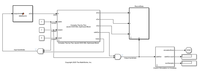
Implement HDL Optimized Two-by-Two Jacobi SVD in Simulink Blocks
The RealTwoByTwoSVDModel and ComplexTwoByTwoSVDModel models contain blocks that implement the real and complex two-by-two SVD algorithms, respectively, optimized for HDL applications. These blocks use the AMBA AXI handshake protocol. The valid/ready handshake process is used to transfer data and control information. This two-way control mechanism allows both the manager and subordinate to control the rate at which information moves between manager and subordinate. A valid signal indicates when data is available. The ready signal indicates that the block can accept the data. Transfer of data occurs only when both the valid and ready signals are high.
Open Model
Open the model corresponding to the specified complexity value.
switch complexity
    case 'real'
        model = 'RealTwoByTwoSVDModel';
    case 'complex'
        model = 'ComplexTwoByTwoSVDModel';
    otherwise
        model = 'RealTwoByTwoSVDModel';
end

open_system(model);
Configure Model Workspace and Run Simulation
Use the fixed.example.setModelWorkspace helper function to configure the model workspace. Run the simulation.
fixed.example.setModelWorkspace(model,'A',A,'numSamples',numSamples);
out = sim(model);
Verify Block Output
Verify that the output of the block is bit-exact with the output of the MATLAB implementation.
UBitExact = ispropequal(out.U,U_fixed)
UBitExact = logical
   1
sBitExact = ispropequal(out.s,S_fixed)
sBitExact = logical
   1
VBitExact = ispropequal(out.V,V_fixed)
VBitExact = logical
   1
Benchmark Latency
This block uses pipelined architecture.
For real 16-bit signed input, the input and output rate is 19 clocks per matrix, and the latency is 44 clocks.
For complex 16-bit signed input, the input and output rate is 50 clocks per matrix, and the latency is 93 clocks.
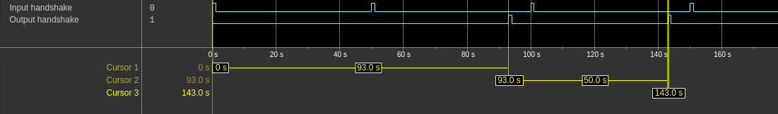
In this example plot:
Cursor 1 points to the input time of first matrix.
Cursor 2 points to the output time of the SVD corresponding to the first matrix.
Cursor 3 points to the output time of the SVD corresponding to the second matrix.
After initialization of 93 clocks, this block can provide SVD at every 50 clocks.
Measure Simulated Latency
Measure the simulated latency.
InputHandshakeHistory = out.logsout.get('Input handshake').Values.Data;
OutputHandshakeHistory = out.logsout.get('Output handshake').Values.Data;
tDataIn = find(InputHandshakeHistory == 1);
tDataOut = find(OutputHandshakeHistory == 1);
simulatedInputRate = diff(tDataIn)
simulatedInputRate = 3×1

    50
    50
    50
simulatedOutputRate = diff(tDataIn)
simulatedOutputRate = 3×1

    50
    50
    50
simulatedLatency = tDataOut - tDataIn(1:numSamples)
simulatedLatency = 3×1

    93
    93
    93
Hardware Resource Utilization
Both blocks in this example support HDL code generation using the Simulink® HDL Workflow Advisor. For an example, see HDL Code Generation and FPGA Synthesis from Simulink Model (HDL Coder) and Implement Digital Downconverter for FPGA (DSP HDL Toolbox).
This example data was generated by synthesizing the block on a AMD® Zynq®-UltraScale+ RFSoC ZCU111. The synthesis tool was Vivado® v2024.1.
These parameters were used for synthesis:
Input data type:
sfix16_En10Target frequency: 350 MHz
These tables show the synthesis resource utilization results and timing summary for the Real Two-by-Two Jacobi SVD HDL Optimized block.
Resource | Usage | Available | Utilization (%) |
Slice LUTs | 1416 | 425280 | 0.33 |
Slice Registers | 1107 | 850560 | 0.13 |
DSPs | 20 | 4272 | 0.51 |
Block RAM Tile | 0 | 0 | 0.00 |
URAM | 0 | 80 | 0.00 |
Value | |
Requirement | 2.5 ns (350 MHz) |
Data Path Delay | 2.355 ns |
Slack | 0.484 ns |
Clock Frequency | 421.38 MHz |
These tables show the synthesis resource utilization results and timing summary for the Complex Two-by-Two Jacobi SVD HDL Optimized block.
Resource | Usage | Available | Utilization (%) |
Slice LUTs | 6717 | 425280 | 1.58 |
Slice Registers | 3475 | 850560 | 0.41 |
DSPs | 32 | 4272 | 0.75 |
Block RAM Tile | 0 | 0 | 0.00 |
URAM | 0 | 80 | 0.00 |
Value | |
Requirement | 2.8571 ns (350 MHz) |
Data Path Delay | 2.683 ns |
Slack | 0.156 ns |
Clock Frequency | 370.21 MHz |
References
[1] Cavallaro, Joseph R., and Franklin T. Luk, "CORDIC Arithmetic for an SVD Processor." Journal of Parallel and Distributed Computing 5, no. 3 (June 1988): 271-90. https://doi.org/10.1016/0743-7315(88)90021-4.
[2] Hager, William W. "Bidiagonalization and Diagonalization." Computers & Mathematics with Applications 14, no. 7 (1987): 561–72. https://doi.org/10.1016/0898-1221(87)90051-4.
See Also
Square Jacobi SVD HDL Optimized | Non-Square Jacobi SVD HDL Optimized
Topics
- Implement HDL Optimized SVD in Feedforward Fashion Without Backpressure
- Implement HDL Optimized SVD with Backpressure Signal and HDL FIFO Block
- Compute SVD of Non-Square Matrices Using Square Jacobi SVD HDL Optimized Block by Forming Covariance Matrices
- Implement HDL Optimized SVD for Non-Square Matrix with Scalar Input and Simplified AXI4 Protocol
- Compute SVD of Non-Square Matrices Using Square Jacobi SVD HDL Optimized Block by Forming Covariance Matrices