Main Content

ratecurve

R2026b

Create ratecurve object for interest-rate curve from dates and data

Description

Build a ratecurve object using ratecurve.

After creating a ratecurve object, you can use the associated object functions forwardrates, discountfactors, and zerorates.

Note

If you have the interest-rate term structure obtained previously from the intenvset or toRateSpec function for an IRDataCurve or IRFunctionCurve object, refer to Workflow for Creating and Analyzing a ratecurve and parametercurve.

To price a Swap, FixedBond, FloatBond, FRA, or Deposit instrument, you must create a ratecurve object and then create a Discount pricer object.

For more detailed information on this workflow, see Get Started with Workflows Using Object-Based Framework for Pricing Financial Instruments.

For more information on the available instruments, models, and pricing methods, see Choose Instruments, Models, and Pricers.

Creation

Description

ratecurve_obj = ratecurve(Type,Settle,Dates,Rates) creates a ratecurve object.

example

ratecurve_obj = ratecurve(___,Name=Value) creates a ratecurve object using name-value pairs and any of the arguments in the previous syntax. For example, myRC = ratecurve("zero",Settle,ZeroDates,ZeroRates,Compounding=2,Basis=5,InterpMethod="pchip",ShortExtrapMethod="linear",LongExtrapMethod="cubic") creates a ratecurve object for a zero curve. You can specify multiple name-value pair arguments.

example

Input Arguments

expand all

Type of interest-rate curve, specified as "zero", "forward", or "discount".

Settlement date, specified as a datetime scalar or string scalar.

To support existing code, ratecurve also accepts serial date numbers as inputs, but they are not recommended.

If you use a date string, the format must be recognizable by the datetime function because the Settle property is stored as a datetime.

Dates corresponding to the rate data, specified as a datetime vector or string vector.

To support existing code, ratecurve also accepts serial date numbers as inputs, but they are not recommended.

If you use a date string, the format must be recognizable by the datetime function because the Dates property is stored as a datetime.

Interest-rate data for the curve, specified as a numeric vector.

Name-Value Arguments

expand all

Specify optional pairs of arguments as Name1=Value1,...,NameN=ValueN, where Name is the argument name and Value is the corresponding value. Name-value arguments must appear after other arguments, but the order of the pairs does not matter.

Before R2021a, use commas to separate each name and value, and enclose Name in quotes.

Example: myRC = ratecurve("zero",Settle,ZeroDates,ZeroRates,Compounding=2,Basis=5,InterpMethod="pchip",ShortExtrapMethod="linear",LongExtrapMethod="cubic")

Compounding frequency, specified as -1, 0, 1, 2, 3, 4, 6, or 12.

Day count basis, specified as one of these values:

  • 0 — actual/actual

  • 1 — 30/360 (SIA)

  • 2 — actual/360

  • 3 — actual/365

  • 4 — 30/360 (PSA)

  • 5 — 30/360 (ISDA)

  • 6 — 30/360 (European)

  • 7 — actual/365 (Japanese)

  • 8 — actual/actual (ICMA)

  • 9 — actual/360 (ICMA)

  • 10 — actual/365 (ICMA)

  • 11 — 30/360E (ICMA)

  • 12 — actual/365 (ISDA)

  • 13 — BUS/252

For more information, see Basis.

Interpolation method, specified as "linear", "cubic", "next", "previous", "pchip", "v5cubic", "makima", "spline", "log-linear", "log-pchip", "log-makima", or "log-spline".

The "log-linear", "log-pchip", "log-makima", and "log-spline" methods perform interpolation in the logarithmic domain. The function applies the corresponding base interpolation method ("linear", "pchip", "makima", or "spline") to the natural logarithm of the rate data and then exponentiates the result. These methods are commonly used in fixed-income applications where interpolation on discount factors or rates benefits from log-space smoothness.

For more information on interpolation methods, see interp1.

Extrapolation method for data before first data, specified as "linear", "cubic", "next", "previous", "pchip", "v5cubic", "makima", "spline", "log-linear", "log-pchip", "log-makima", or "log-spline".

The "log-linear", "log-pchip", "log-makima", and "log-spline" methods perform interpolation in the logarithmic domain. The function applies the corresponding base interpolation method ("linear", "pchip", "makima", or "spline") to the natural logarithm of the rate data and then exponentiates the result. These methods are commonly used in fixed-income applications where interpolation on discount factors or rates benefits from log-space smoothness.

For more information on interpolation methods, see interp1.

Extrapolation method for data after last data, specified as "linear", "cubic", "next", "previous", "pchip", "v5cubic", "makima", "spline", "log-linear", "log-pchip", "log-makima", or "log-spline".

The "log-linear", "log-pchip", "log-makima", and "log-spline" methods perform interpolation in the logarithmic domain. The function applies the corresponding base interpolation method ("linear", "pchip", "makima", or "spline") to the natural logarithm of the rate data and then exponentiates the result. These methods are commonly used in fixed-income applications where interpolation on discount factors or rates benefits from log-space smoothness.

For more information on interpolation methods, see interp1.

Output Arguments

expand all

Rate curve, returned as a ratecurve object.

Properties

expand all

Type of interest-rate curve, returned as "zero", "forward", or "discount".

Data Types: string

Compounding frequency, returned as -1, 0, 1, 2, 3, 4, 6, or 12.

Data Types: double

Day count basis, returned as one of these values:

  • 0 — actual/actual

  • 1 — 30/360 (SIA)

  • 2 — actual/360

  • 3 — actual/365

  • 4 — 30/360 (PSA)

  • 5 — 30/360 (ISDA)

  • 6 — 30/360 (European)

  • 7 — actual/365 (Japanese)

  • 8 — actual/actual (ICMA)

  • 9 — actual/360 (ICMA)

  • 10 — actual/365 (ICMA)

  • 11 — 30/360E (ICMA)

  • 12 — actual/365 (ISDA)

  • 13 — BUS/252

For more information, see Basis.

Data Types: double

Dates corresponding to the rate data, returned as a datetime vector.

Data Types: datetime

Interest-rate data for the curve, returned as a numeric vector.

Data Types: double

Settlement date, returned as a datetime scalar.

Data Types: datetime

Interpolation method, returned as "linear", "cubic", "next", "previous", "pchip", "v5cubic", "makima", "spline", "log-linear", "log-pchip", "log-makima", or "log-spline".

Data Types: string

Extrapolation method for data before first data, returned as "linear", "cubic", "next", "previous", "pchip", "v5cubic", "makima", "spline", "log-linear", "log-pchip", "log-makima", or "log-spline".

Data Types: string

Extrapolation method for data after last data, specified as "linear", "cubic", "next", "previous", "pchip", "v5cubic", "makima", "spline", "log-linear", "log-pchip", "log-makima", or "log-spline".

Data Types: string

Object Functions

forwardratesCalculate forward rates for ratecurve object
discountfactorsCalculate discount factors for a ratecurve object
zeroratesCalculate zero rates for ratecurve object
irbootstrapBootstrap interest-rate curve from market data

Examples

collapse all

Create a ratecurve object using the ratecurve function.

Settle = datetime(2018,9,15);
Type = "zero";
ZeroTimes = [calmonths(6) calyears([1 2 3 4 5 7 10 20 30])]';
ZeroRates = [0.0052 0.0055 0.0061 0.0073 0.0094 0.0119 0.0168 0.0222 0.0293 0.0307]';
ZeroDates = Settle + ZeroTimes;
 
myRC = ratecurve("zero",Settle,ZeroDates,ZeroRates,Compounding=2,Basis=5,InterpMethod="pchip",ShortExtrapMethod="linear",LongExtrapMethod="pchip")
myRC = 
  ratecurve with properties:

                 Type: "zero"
          Compounding: 2
                Basis: 5
                Dates: [10×1 datetime]
                Rates: [10×1 double]
               Settle: 15-Sep-2018
         InterpMethod: "pchip"
    ShortExtrapMethod: "linear"
     LongExtrapMethod: "pchip"

Create a ratecurve object using log-linear interpolation and compare discount factors with a standard linear interpolation curve.

Define the settlement date, zero rate data, and corresponding dates. Then create a ratecurve object using standard linear interpolation.

Type = "zero";
Settle = datetime(2026,2,11);
Dates = Settle + [calmonths([1 2 3 6]) calyears([1 2 3 5 7 10 20 30])]';
Rates = [3.71 3.73 3.70 3.60 3.47 3.52 3.55 3.75 3.96 4.18 4.76 4.82]'/100;
Compounding = -1;
Basis = 3;

RC_linear = ratecurve(Type,Settle,Dates,Rates,Compounding=Compounding,Basis=Basis,InterpMethod="linear");

Compute the discount factors from the linear curve.

DF = discountfactors(RC_linear,Dates);

Create a second ratecurve object using the discount factors as inputs and specify log-linear interpolation. Log-linear interpolation operates in the logarithmic domain, which helps preserve positivity of implied forward rates.

RC_loglinear = ratecurve("discount",Settle,Dates,DF,InterpMethod="log-linear",Compounding=Compounding,Basis=Basis);

Define a finer set of query dates for comparison.

QueryDates = Settle + calmonths(1:360)';

Compute discount factors from both curves at the query dates.

DF_linear = discountfactors(RC_linear,QueryDates);
DF_loglinear = discountfactors(RC_loglinear,QueryDates);

Plot the discount factors to compare the two interpolation methods.

figure
plot(QueryDates,DF_linear,QueryDates,DF_loglinear)
legend("Linear","Log-Linear")
xlabel("Date")
ylabel("Discount Factor")
title("Discount Factor Comparison: Linear vs. Log-Linear Interpolation")
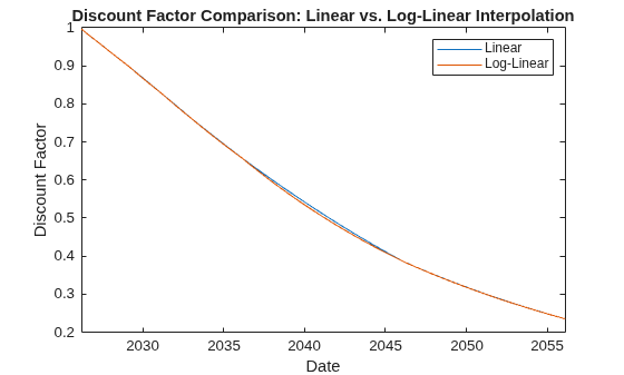
Figure contains an axes object. The axes object with title Discount Factor Comparison: Linear vs. Log-Linear Interpolation, xlabel Date, ylabel Discount Factor contains 2 objects of type line. These objects represent Linear, Log-Linear.

Version History

Introduced in R2020a

expand all