Machine Learning for Statistical Arbitrage II: Feature Engineering and Model Development
This example creates a continuous-time Markov model of limit order book (LOB) dynamics, and develops a strategy for algorithmic trading based on patterns observed in the data. It is part of a series of related examples on machine learning for statistical arbitrage (see Machine Learning Applications).
Exploratory Data Analysis
To predict the future behavior of a system, you need to discover patterns in historical data. The vast amount of data available from exchanges, such as NASDAQ, poses computational challenges while offering statistical opportunities. This example explores LOB data by looking for indicators of price momentum, following the approach in [4].
Raw Data
Load LOBVars.mat, the preprocessed LOB data set of the NASDAQ security INTC, which is included with the Financial Toolbox™ documentation.
load LOBVarsThe data set contains the following information for each order: the arrival time t (seconds from midnight), level 1 asking price MOAsk, level 1 bidding price MOBid, midprice S, and imbalance index I.
Create a plot that shows the intraday evolution of the LOB imbalance index I and midprice S.
figure

t.Format = "hh:mm:ss";

yyaxis left
plot(t,I)
ylabel("Imbalance Index")

yyaxis right
plot(t,S/10000,'LineWidth',2)
ylabel("Midprice (Dollars)")

xlabel("Time")

title('Exchange Data: One Day')
legend(["Imbalance","Midprice"],'Location','NE')
grid on
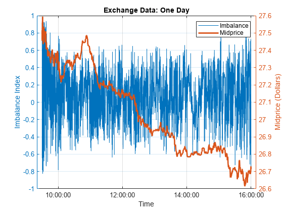
At this scale, the imbalance index gives no indication of future changes in the midprice.
To see more detail, limit the time scale to one minute.
timeRange = seconds([36000 36060]); % One minute after 10 AM, when prices were climbing
xlim(timeRange)
legend('Location','SE')
title("Exchange Data: One Minute")
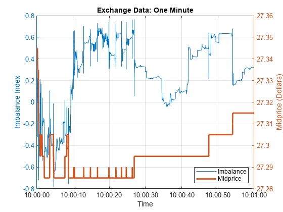
At this scale, sharp departures in the imbalance index align with corresponding departures in the midprice. If the relationship is predictive, meaning imbalances of a certain size forecast future price movements, then quantifying the relationship can provide statistical arbitrage opportunities.
Plot a histogram of the interarrival times in the LOB.
DT = diff(t); % Interarrival Times
DT.Format = "s";

figure
binEdges = seconds(0.01:0.01:1);
histogram(DT,binEdges)
xlabel("Seconds")
ylabel("Number of Orders")
title("LOB Interarrival Times")
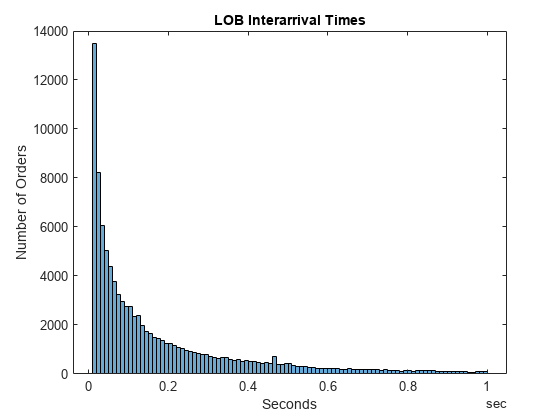
Interarrival times follow the characteristic pattern of a Poisson process.
Compute the average wait time between orders by fitting an exponential distribution to the interarrival times.
DTAvg = expfit(DT)
DTAvg = duration
   0.040273 sec
Smoothed Data
The raw imbalance series I is erratic. To identify the most significant dynamic shifts, introduce a degree of smoothing dI, which is the number of backward ticks used to average the raw imbalance series.
dI = 10; % Hyperparameter
dTI = dI*DTAvg
dTI = duration
0.40273 sec
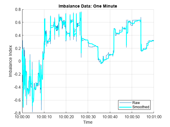
The setting corresponds to an interval of 10 ticks, or about 0.4 seconds on average. Smooth the imbalance indices over a trailing window.
sI = smoothdata(I,'movmean',[dI 0]);Visualize the degree of smoothing to assess the volatility lost or retained.
figure
hold on
plot(t,I)
plot(t,sI,'c','LineWidth',2)
hold off

xlabel("Time")
xlim(timeRange)
ylabel("Imbalance Index")
title("Imbalance Data: One Minute")
legend(["Raw","Smoothed"],'Location','SE')
grid on
Discretized Data
To create a Markov model of the dynamics, collect the smoothed imbalance index sI into bins, discretizing it into a finite collection of states rho (). The number of bins numBins is a hyperparameter.
numBins = 3; % Hyperparameter
binEdges = linspace(-1,1,numBins+1);
rho = discretize(sI,binEdges);
To model forecast performance, aggregate prices over a leading window. The number of ticks in a window dS is a hyperparameter.
dS = 20; % Hyperparameter
dTS = dS*DTAvg
dTS = duration
0.80547 sec
The setting corresponds to an interval of 20 ticks, or about 0.8 seconds on average. Discretize price movements into three states DS () given by the sign of the forward price change.
DS = NaN(size(S));
shiftS = S(dS+1:end);
DS(1:end-dS) = sign(shiftS-S(1:end-dS));
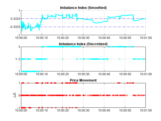
Visualize the discretized data.
figure

subplot(3,1,1)
hold on
plot(t,sI,'c','LineWidth',2)
for i = 2:numBins
    yline(binEdges(i),'b--');
end
hold off
xlim(timeRange)
ylim([-1 1])
yticks(binEdges)
title("Imbalance Index (Smoothed)")
grid on

subplot(3,1,2)
plot(t,rho,'co','MarkerSize',3)
xlim(timeRange)
ylim([1 numBins])
yticks(1:numBins)
ylabel("\rho")
title("Imbalance Index (Discretized)")
grid on

subplot(3,1,3)
plot(t,DS,'ro','MarkerSize',3)
xlim(timeRange)
ylim([-1 1])
yticks([-1 0 1])
ylabel("\DeltaS")
title("Price Movement")
grid on
Continuous Time Markov Process
Together, the state of the LOB imbalance index rho () and the state of the forward price movement DS () describe a two-dimensional continuous-time Markov chain (CTMC). The chain is modulated by the Poisson process of order arrivals, which signals any transition among the states.
To simplify the description, give the two-dimensional CTMC a one-dimensional encoding into states phi ().
numStates = 3*numBins; % numStates(DS)*numStates(rho)

phi = NaN(size(t));
for i = 1:length(t)
    switch DS(i)
        case -1
            phi(i) = rho(i);
        case 0
            phi(i) = rho(i) + numBins;
        case 1
            phi(i) = rho(i) + 2*numBins;
    end
end
Successive states of , and the component states and proceed as follows.
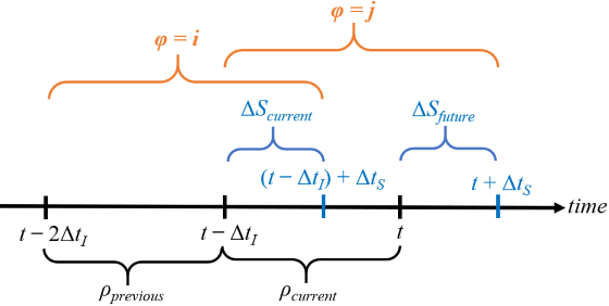
Hyperparameters dI () and dS () determine the size of a rolling state characterizing the dynamics. At time , the process transitions from to (or holds in the same state if ).
Estimate Process Parameters
Execution of the trading strategy at any time is based on the probability of being in a particular state, conditional on the current and previous values of the other states. Following [3] and [4], determine empirical transition probabilities, and then assess them for predictive power.
% Transition counts

C = zeros(numStates);
for i = 1:length(phi)-dS-1
    C(phi(i),phi(i+1)) = C(phi(i),phi(i+1))+1;
end

% Holding times

H = diag(C);

% Transition rate matrix (infinitesimal generator)

G = C./H;
v = sum(G,2);
G = G + diag(-v);

% Transition probability matrix (stochastic for all dI)

P = expm(G*dI); % Matrix exponential
To obtain a trading matrix Q containing as in [4], apply Bayes’ rule,
.
The numerator is the transition probability matrix P. Compute the denominator PCond.
PCond = zeros(size(P));
phiNums = 1:numStates;
modNums = mod(phiNums,numBins);
for i = phiNums
    for j = phiNums
        idx = (modNums == modNums(j));
        PCond(i,j) = sum(P(i,idx));
    end
end

Q = P./PCond;
Display Q in a table. Label the rows and columns with composite states .
binNames = string(1:numBins);
stateNames = ["("+binNames+",-1)","("+binNames+",0)","("+binNames+",1)"];
QTable = array2table(Q,'RowNames',stateNames,'VariableNames',stateNames)
QTable=9×9 table
               (1,-1)      (2,-1)       (3,-1)       (1,0)      (2,0)      (3,0)       (1,1)        (2,1)       (3,1)
              ________    _________    _________    _______    _______    _______    _________    _________    ________

    (1,-1)     0.59952      0.30458      0.19165    0.39343    0.67723     0.7099    0.0070457     0.018196    0.098447
    (2,-1)     0.74092      0.58445      0.40023    0.25506    0.41003    0.56386    0.0040178    0.0055189    0.035914
    (3,-1)     0.79895      0.60866      0.55443    0.19814      0.385    0.42501    0.0029096    0.0063377    0.020554
    (1,0)     0.094173     0.036014     0.019107    0.88963    0.91688    0.75192     0.016195     0.047101     0.22897
    (2,0)      0.12325     0.017282     0.015453    0.86523    0.96939     0.9059     0.011525     0.013328    0.078648
    (3,0)       0.1773      0.02616     0.018494    0.81155    0.95359    0.92513     0.011154     0.020252    0.056377
    (1,1)     0.041132    0.0065127    0.0021313    0.59869    0.39374    0.21787      0.36017      0.59975        0.78
    (2,1)     0.059151    0.0053554    0.0027769    0.65672    0.42325    0.26478      0.28413       0.5714     0.73244
    (3,1)     0.095832     0.010519    0.0051565     0.7768     0.6944     0.3906      0.12736      0.29508     0.60424
Rows are indexed by (). Conditional probabilities for each of the three possible states of are read from the corresponding column, conditional on .
Represent Q with a heatmap.
figure
imagesc(Q)
axis equal tight
hCB = colorbar;
hCB.Label.String = "Prob(\DeltaS_{future} | \rho_{previous},\rho_{current},\DeltaS_{current})";
xticks(phiNums)
xticklabels(stateNames)
xlabel("(\rho_{current},\DeltaS_{future})")
yticks(phiNums)
yticklabels(stateNames)
ylabel("(\rho_{previous},\DeltaS_{current})")
title("Trading Matrix")

The bright, central 3 x 3 square shows that in most transitions, tick to tick, no price change is expected (). Bright areas in the upper-left 3 x 3 square (downward price movements ) and lower-right 3 x 3 square (upward price movements ) show evidence of momentum, which can be leveraged in a trading strategy.
You can find arbitrage opportunities by thresholding Q above a specified trigger probability. For example:
trigger = 0.5;
QPattern = (Q > trigger)
QPattern = 9×9 logical array

   1   0   0   0   1   1   0   0   0
   1   1   0   0   0   1   0   0   0
   1   1   1   0   0   0   0   0   0
   0   0   0   1   1   1   0   0   0
   0   0   0   1   1   1   0   0   0
   0   0   0   1   1   1   0   0   0
   0   0   0   1   0   0   0   1   1
   0   0   0   1   0   0   0   1   1
   0   0   0   1   1   0   0   0   1
The entry in the (1,1) position shows a chance of more than 50% that a downward price movement () will be followed by another downward price movement (), provided that the previous and current imbalance states are both 1.
A Trading Strategy?
Q is constructed on the basis of both the available exchange data and the hyperparameter settings. Using Q to inform future trading decisions depends on the market continuing in the same statistical pattern. Whether the market exhibits momentum in certain states is a test of the weak-form Efficient Market Hypothesis (EMH). For heavily traded assets, such as the one used in this example (INTC), the EMH is likely to hold over extended periods, and arbitrage opportunities quickly disappear. However, failure of EMH can occur in some assets over short time intervals. A working trading strategy divides a portion of the trading day, short enough to exhibit a degree of statistical equilibrium, into a training period for estimating Q, using optimal hyperparameter settings and a validation period on which to trade. For an implementation of such a strategy, see Machine Learning for Statistical Arbitrage III: Training, Tuning, and Prediction.
Summary
This example begins with raw data on the LOB and transforms it into a summary (the Q matrix) of statistical arbitrage opportunities. The analysis uses the mathematics of continuous-time Markov chain models, first in recognizing the Poisson process of LOB interarrival times, then by discretizing data into two-dimensional states representing the instantaneous position of the market. A description of state transitions, derived empirically, leads to the possibility of an algorithmic trading strategy.
References
[1] Cartea, Álvaro, Sebastian Jaimungal, and Jason Ricci. "Buy Low, Sell High: A High-Frequency Trading Perspective." SIAM Journal on Financial Mathematics 5, no. 1 (January 2014): 415–44. https://doi.org/10.1137/130911196.
[2] Guilbaud, Fabien, and Huyen Pham. "Optimal High-Frequency Trading with Limit and Market Orders." Quantitative Finance 13, no. 1 (January 2013): 79–94. https://doi.org/10.1080/14697688.2012.708779.
[3] Norris, J. R. Markov Chains. Cambridge, UK: Cambridge University Press, 1997.
[4] Rubisov, Anton D. "Statistical Arbitrage Using Limit Order Book Imbalance." Master's thesis, University of Toronto, 2015.