Deep Reinforcement Learning for Optimal Trade Execution
This example shows how to use the Reinforcement Learning Toolbox™ and Deep Learning Toolbox™ to design agents for optimal trade execution.
Introduction
Optimal trade execution seeks to minimize trading costs when selling or buying a set number of stock shares over a certain time horizon within the trading day. Optimization is necessary because executing trades too quickly results in suboptimal prices due to market impact, while executing trades too slowly results in exposure to the risk of adverse price changes or the inability to execute all trades within the time horizon. This optimization affects nearly all trading strategies and portfolio management practices, since minimizing trading costs is directly linked to profitability that is related to buying or selling decisions. Also, brokers compete to provide better trade order execution, and many jurisdictions legally require brokers to provide the best execution for their clients. Early studies by Bertsimas and Lo [1] and Almgren and Chriss [2] derived analytical solutions for the optimal trade execution problem by assuming a model for the underlying prices. Later, Nevmyvaka et al. [3] demonstrated that the use of reinforcement learning (RL) for optimal execution did not require making assumptions about the market micro-structure. More recent studies use deep reinforcement learning, which combines reinforcement learning (RL) with deep learning, for optimal trade execution (Ning et al. [4], Lin and Beling [5,6]). This approach overcomes the limitations of Q-learning as noted by Nevmyvaka et al. [3].
This example uses deep reinforcement learning to design and train two deep Q-network (DQN) agents for optimal trade execution. One DQN agent is for sell trades and the other agent is for buy trades.
Data
This example uses the intraday trading data on Intel Corporation stock (INTC) provided by LOBSTER [7] and included with Financial Toolbox™. While the reinforcement learning for optimal execution literature typically uses trading data over one year or more to train and test RL agents [3,4,5,6], in this proof-of-concept example you use a shorter data set, which you can expand for further study. The intraday trading data on the Intel stock (INTC_2012-06-21_34200000_57600000_orderbook_5.csv) contains limit order book data over 6.5 hours, including bid and ask prices as well as corresponding shares for 5 levels. This data is sampled at 5 second intervals to create 390 one minute trading horizons, such that each trading horizon contains 12 steps at five second intervals. Out of these 390 horizons, you use 293 horizons (about 75 percent) to train the agents and the remaining 97 horizons (about 25 percent) to test the agents.
Baseline Trade Execution Algorithm
An agent's performance must be compared with a baseline trade execution algorithm. For this example, the baseline trade execution algorithm is the time-weighted average price (TWAP) policy. Under this policy, the total trading shares are divided equally over the trading horizon, so that the same number of shares are traded at each time step. In contrast, the original paper by Nevmyvaka et al. [3] used a "submit and leave" policy as the baseline, where a limit order is placed at a fixed price for the entire trading shares for the entire horizon, and any remaining unfilled shares are traded with a market order at the last step. However, the TWAP baseline was adopted in later studies [4,5,6], since it has become more popular in recent years with increasing use of algorithmic trading, and it is also a highly effective strategy that is thought to be optimal when the price movement follows a Brownian motion [4,5,6].
Agents
Different types of agents are used in the reinforcement learning for optimal execution studies, including Q-learning [3], DQN [4,5], and PPO [6] agents. In this example, you design and train DQN agents using the Reinforcement Learning Designer (Reinforcement Learning Toolbox) after creating separate training environments for sell trades and buy trades. These DQN agents only have a critic without an actor, and they use the default setting of UseDoubleDQN set to true, while the DiscountFactor is set to 1 due to the short trading horizon [4,5,6]. In addition, the critic network of these agents include a long short-term memory (LSTM) network because the trading data is sequential in time, and LSTM networks are effective in designing agents for optimal execution [6]. For more information on setting options for DQN agents, see rlDQNAgentOptions (Reinforcement Learning Toolbox).
Observation Space
The observation space defines which information (or feature) to provide to the agents at each step. The agents use this observation to decide the next action, based on the policy learned and reinforced by the rewards received after taking the previous actions. Designing a good observation space for the agents is an area of active research in optimal execution studies. You can experiment with different observation spaces, using variables such as the bid-ask spread, the bid or ask volume, price trends, or even the entire limit order book prices and shares [6]. This example uses the following observation variables:
Remaining shares to be traded by the agent in the current trading horizon
Remaining time intervals (steps) left in the current trading horizon
Cumulative implementation shortfall (IS) of agent until the previous step
Current limit order book price divergence from arrival price
The first two observation variables (remaining shares to be traded and remaining time in horizon) are called "private" variables by Nevmyvaka et al. [3], as they only apply to the specific situation of the trading agents, and they do not apply to other market participants. As the agent trained by Nevmyvaka et al. [3] using only "private" variables was able to outperform the "submit and leave" baseline policy, the "private" variables are also used in the subsequent studies [4,5,6].
The third variable, cumulative IS, is a measure of trading cost that the agents seek to minimize. As the name "shortfall" indicates, a lower implementation shortfall implies better trade execution. Technically, Implementation Shortfall should include the opportunity cost of failing to execute all shares within the trading horizon. In this example, as with many of the previously mentioned studies, the Implementation Shortfall is computed under the ending inventory constraint:
For a sell trade, the constraint is to have zero ending inventory, assuming successful liquidation of all shares.
For a buy trade, the constraint is to have full ending inventory, assuming successful purchase of all shares.
Under this ending inventory constraint, Implementation Shortfall is computed as follows:
For a sell trade:
For a buy trade:
The arrival price is the first bid or ask price observed at the beginning of the trade horizon. If Implementation Shortfall is positive, it implies that the average executed price was worse than the arrival price, while a negative Implementation Shortfall implies that the average executed price was better than the arrival price. The cumulative Implementation Shortfall from the beginning of the trade horizon until the previous step reflects the trading cost incurred by the agent in the past, and it serves as the third observation variable.
The last observation variable is the current price divergence from arrival price. This variable reflects the current market condition and it is measured as the difference between the arrival price and the average price of the first two levels of the current limit order book (LOB).
For a sell trade:
For a buy trade:
A positive price divergence implies more favorable current trading conditions than the arrival price, and a negative divergence less favorable conditions.
Action Space
The action space is defined as the possible number of shares traded at each step. For a TWAP policy, the only possible action at each step is to trade a constant number of shares computed as the total trading shares divided by the number of steps in the horizon. Meanwhile, the agents in this example choose from 39 possible actions that are mostly evenly spaced, ranging from trading 0 shares to trading twice the number of shares as the corresponding TWAP trade.
For both TWAP trades and agent trades, you enforce ending inventory constraints so that if the target ending inventory is not met by the last step of the horizon, the action for the last step is to:
Sell any remaining shares in the inventory for a Sell trade.
Buy any missing shares in the inventory for a Buy trade.
Also, you place limits on the agent actions to take advantage of price divergence and to prevent selling more than the available shares in the inventory or buying more than the target number of shares.
Reward
The reward is another important aspect of agent design, as agents learn their policies at each step using the rewards received after taking the previous actions. Research on reward design shows wide variations in optimal execution, and you can experiment with different rewards. Since the agent performance is measured against the baseline using Implementation Shortfall, many studies use Implementation Shortfalls directly in the rewards, while others use related quantities. Some studies use the proceeds from the trade as the reward [3], while others also impose a penalty for trading many shares too quickly [4]. Another study uses an elaborately shaped reward algorithm that is designed to use the TWAP policy most of the time, while encouraging the agent to deviate from the TWAP policy only when it is advantageous to do so [5]. If there is enough data, the reward may be given sparsely, only at the end of each horizon rather than at each step [6]. In this example, the data size is small, so you give the reward at each step and design it so that the reward at each step approximates the expected reward at the end of the horizon.
Specifically, you use a reward that compares the Implementation Shortfall of the TWAP baseline against that of the agent at each step, while also taking into account the penalty for the approximate Implementation Shortfall of the remaining unexecuted shares based on the current limit order book. The reward is also scaled based on the current time relative to the end of the horizon.
is the reward at time step
is the Implementation Shortfall of TWAP from the beginning of the horizon until time step
is the approximate Implementation Shortfall of TWAP from time step to the end of the horizon at time step
is the Implementation Shortfall of the agent from the beginning of horizon until time step
is the approximate Implementation Shortfall of the agent from time step to the end of the horizon at time step
Since the agent performance is ultimately measured against the baseline using Implementation Shortfall at the end of the horizon at time step , and the approximate reward becomes more accurate as approaches , has a scaling factor so that its magnitude increases as approaches . At time step , the reward becomes .
Performance Analysis
You measure agent performance against the TWAP baseline using Implementation Shortfall (IS), by computing the following for all horizons:
IS total outperformance of agent over TWAP — Sum of
IS total-gain-to-loss ratio (TGLR) — Ratio of total positive over total negative magnitudes
IS gain-to-loss ratio (GLR) — Ratio of mean positive over mean negative magnitudes
Workflow Organization
The workflow in this example is:
- LOBSTER Message Data — Contains time stamps
- LOBSTER Limit Order Book Data — Contains bid and ask prices and corresponding shares
- TWAP Baseline
- Train the DQN Agent
- Test the DQN Agent
- Summary of Selling Results
-
executeTWAPTrades— Executes TWAP Baseline trades and computes IS-
RL_OptimalExecution_LOB_ResetFcn— Reset function for training and testing environments-
RL_OptimalExecution_LOB_StepFcn— Step function for training and testing environments-
tradeLOB— Executes trades on current limit order book-
endingInventoryIS— Computes IS with ending inventory constraints-
ISTGLR— Computes total-gain-to-loss ratio and gain-to-loss ratio for IS
Load and Prepare Message Data
Extract the LOBSTER data files from the ZIP file included with Financial Toolbox™. The expanded files include two CSV files of data and the text file LOBSTER_SampleFiles_ReadMe.txt.
unzip("LOBSTER_SampleFile_INTC_2012-06-21_5.zip");The limit order book file contains the bid and ask prices and corresponding shares for five levels, while the message file contains the description of the limit order book data including time stamps.
LOBFileName = 'INTC_2012-06-21_34200000_57600000_orderbook_5.csv'; % Limit Order Book Data file
MSGFileName = 'INTC_2012-06-21_34200000_57600000_message_5.csv'; % Message file (description of data)
Load the message file and define the time at the start and end of trading hours as seconds after midnight.
TradeMessage = readmatrix(MSGFileName);
StartTradingSec   = 9.5*60*60;  % Starting time 9:30 in seconds after midnight
EndTradingSec     = 16*60*60;   % Ending time 16:00 in seconds after midnight
Define the trading interval as five seconds and pick message index values corresponding to the five-second intervals.
TradingIntervalSec = 5; % Trading interval length in seconds
IntervalBoundSec = (StartTradingSec:TradingIntervalSec:EndTradingSec)';
MessageSampleIdx = zeros(size(IntervalBoundSec));
k1 = 1;
for k2 = 1:size(TradeMessage,1)
    if TradeMessage(k2,1) >= IntervalBoundSec(k1)
        MessageSampleIdx(k1) = k2;
        k1 = k1+1;
    end
end
MessageSampleIdx(end) = length(TradeMessage);
Load and Prepare Limit Order Book Data
Load the limit order book data and define the number of levels in the limit order book.
LOB = readmatrix(LOBFileName);
NumLevels = 5;
Since LOBSTER stores prices in units of 10,000 dollars, convert the prices in the limit order book data into dollars by dividing by 10000.
LOB(:,1:2:(4*NumLevels)) = LOB(:,1:2:(4*NumLevels))./10000;
Using the message index values obtained previously, sample the limit order book at 5 second intervals.
SampledBook = LOB(MessageSampleIdx(2:end),1:NumLevels*4);
Define a one minute (60 seconds) trading horizon and compute the total number of intervals over 6.5 hours of trading data.
TradingHorizon = 1*60;
TotalNumIntervals = length(MessageSampleIdx(2:end));
TotalNumHorizons = 6.5*60*60/TradingHorizon;
The number of intervals per horizon is computed by dividing the total number of intervals by the total number of horizons.
NumIntervalsPerHorizon = round(TotalNumIntervals/TotalNumHorizons);
Allocate 75 percent of data for training and 25 percent for testing.
NumTrainingHorizons = round(TotalNumHorizons*0.75);
NumTestingHorizons = TotalNumHorizons - NumTrainingHorizons;
NumTrainingSteps = NumTrainingHorizons*NumIntervalsPerHorizon;
NumTestingSteps = NumTestingHorizons*NumIntervalsPerHorizon;
TrainingLOB = SampledBook(1:NumTrainingSteps,:);
TestingLOB = SampledBook(NumTrainingSteps+1:end,:);
Optimal Execution for Sell Trades
These sections compose the workflow for designing a DQN agent for the optimal execution of sell trades:
Validate Training Environment Reset and Step Functions for Sell Trades
Compute IS Using Trained Agent and Training Data for Sell Trades
Validate Testing Environment Reset and Step Functions for Sell Trades
Compute IS Using Trained Agent and Testing Data for Sell Trades
Display Summary of Training and Testing Results for Sell Trades
Define Settings for Sell Trades
To indicate sell trades, set the BuyTrade logical flag to false.
BuyTrade = false;
Define the total number of shares to sell over the horizon.
TotalTradingShares_Sell = 2738;
TWAP Baseline Analysis on Training Data
Execute TWAP trades and compute Implementation Shortfall (IS) using the executeTWAPTrades function, which uses the tradeLOB function to execute the trades and the endingInventoryIS function to compute IS. These functions are in the Local Functions section.
[IS_TWAP_Horizon_Train_Sell,IS_TWAP_Step_Train_Sell, ...
    InventoryShares_Step_TWAP_Train_Sell,TradingShares_Step_TWAP_Train_Sell] = ...
    executeTWAPTrades(TrainingLOB,NumLevels,TotalTradingShares_Sell, ...
    NumIntervalsPerHorizon,NumTrainingHorizons,BuyTrade);
Plot the implementation shortfall, executed shares, and inventory shares for the TWAP baseline for each step using the training data.
figure
subplot(3,1,1)
bar(1:NumTrainingSteps, IS_TWAP_Step_Train_Sell)
xlabel(strcat("Step number (", num2str(TradingIntervalSec), ...
    " sec intervals, ", num2str(NumTrainingSteps), " steps total.)"))
ylabel("Implementation Shortfall")
title("Implementation Shortfall (TWAP, Training, Sell)")
xlim([0 300])

subplot(3,1,2)
bar(1:NumTrainingSteps, TradingShares_Step_TWAP_Train_Sell)
xlabel(strcat("Step number (", num2str(TradingIntervalSec), ...
    " sec intervals, ", num2str(NumTrainingSteps), " steps total.)"))
ylabel("Executed Shares")
title("Shares Traded at Each Step (TWAP, Training, Sell)")
xlim([0 300])
ylim([0 2000])

subplot(3,1,3)
bar(1:NumTrainingSteps, InventoryShares_Step_TWAP_Train_Sell)
xlabel(strcat("Step number (", num2str(TradingIntervalSec), ...
    " sec intervals, ", num2str(NumTrainingSteps), " steps total.)"))
ylabel("Inventory Shares")
title("Inventory Shares (TWAP, Training, Sell)")
xlim([0 300])
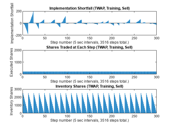
The TWAP executed shares in the middle panel have a flat profile, since the same number of shares are traded at each step. Also, the inventory shares in the bottom panel have a nearly perfect triangular sawtooth pattern, with the number of inventory shares declining linearly at each horizon as the shares are sold. The IS in the top panel sometimes declines to negative values (implying better executions than arrival price) for some horizons, while it increases to positive values (implying worse executions than arrival price) for other horizons.
Set Up RL Training Environment for Sell Trades
The RL environment requires observation and action information, reset function, and a step function.
Define the observation information for the four observation variables.
ObservationDimension = [1 4];
ObservationInfo_Train_Sell = rlNumericSpec(ObservationDimension);
ObservationInfo_Train_Sell.Name = 'Observation Data';
ObservationInfo_Train_Sell.Description = 'RemainingSharesToTrade, RemainingIntervals, IS_Agent, PriceDivergence';
ObservationInfo_Train_Sell.LowerLimit = -inf;
ObservationInfo_Train_Sell.UpperLimit = inf;
Define the environment constants for the training data and the reset function. The function definition for RL_OptimalExecution_LOB_ResetFcn is in the Local Functions section.
EnvConstants_Train_Sell.SampledBook = TrainingLOB;
EnvConstants_Train_Sell.BuyTrade = BuyTrade;
EnvConstants_Train_Sell.TotalTradingShares = TotalTradingShares_Sell;
EnvConstants_Train_Sell.NumIntervalsPerHorizon = NumIntervalsPerHorizon;
EnvConstants_Train_Sell.NumHorizons = NumTrainingHorizons;
EnvConstants_Train_Sell.NumSteps = NumTrainingSteps;
EnvConstants_Train_Sell.NumLevels = NumLevels;
EnvConstants_Train_Sell.IS_TWAP = IS_TWAP_Step_Train_Sell;

ResetFunction_Sell = @() RL_OptimalExecution_LOB_ResetFcn(EnvConstants_Train_Sell);
Define the action information as the number of shares to be traded at each step, ranging from zero shares to twice the number of shares as in TWAP.
NumActions = 39;
LowerActionRange = linspace(0,TradingShares_Step_TWAP_Train_Sell(1), round(NumActions/2));
ActionRange = round([LowerActionRange(1:end-1) ...
    linspace(TradingShares_Step_TWAP_Train_Sell(1), ...
    TradingShares_Step_TWAP_Train_Sell(1)*2,round(NumActions/2))]);

ActionInfo_Sell = rlFiniteSetSpec(ActionRange);
ActionInfo_Sell.Name = 'Trading Action (Number of Shares)';
ActionInfo_Sell.Description = 'Number of Shares to be Traded at Each Time Step';
Define the step function, which computes the rewards and updates the observations at each step. The function definition for RL_OptimalExecution_LOB_StepFcn is in the Local Functions section.
StepFunction_Train_Sell = @(Action,LoggedSignals) ...
    RL_OptimalExecution_LOB_StepFcn(Action,LoggedSignals,EnvConstants_Train_Sell);
Create the environment using the custom function handles defined in this section.
RL_OptimalExecution_Training_Environment_Sell = rlFunctionEnv(ObservationInfo_Train_Sell,ActionInfo_Sell,StepFunction_Train_Sell,ResetFunction_Sell)
Reset!
Reset!
RL_OptimalExecution_Training_Environment_Sell =
  rlFunctionEnv with properties:

     StepFcn: @(Action,LoggedSignals)RL_OptimalExecution_LOB_StepFcn(Action,LoggedSignals,EnvConstants_Train_Sell)
    ResetFcn: @()RL_OptimalExecution_LOB_ResetFcn(EnvConstants_Train_Sell)
        Info: [1×1 struct]
Validate Training Environment Reset and Step Functions for Sell Trades
Before using the created environment, the best practice is to validate the reset and step functions for the environment. Call the reset and step functions to see if they produce reasonable results without errors.
Validate the reset function and the initial observation.
InitialObservation = reset(RL_OptimalExecution_Training_Environment_Sell);
Reset!
InitialObservation
InitialObservation = 1×4

    2738    12    0    0
Validate the step function by monitoring the logged signals and rewards while calling the step functions multiple times. Here, you can see the time interval index increasing at each step and the current inventory shares changing as the trades are executed at each step.
[~,Reward1,~,LoggedSignals1] = step(RL_OptimalExecution_Training_Environment_Sell,TradingShares_Step_TWAP_Train_Sell(1));
LoggedSignals1
LoggedSignals1 = struct with fields:
               IntervalIdx: 1
                HorizonIdx: 1
    CurrentInventoryShares: 2624
              ArrivalPrice: 27.4600
            ExecutedShares: 114
            ExecutedPrices: 27.4600
     HorizonExecutedShares: [60×1 double]
     HorizonExecutedPrices: [60×1 double]
                  IS_Agent: [3516×1 double]
                    Reward: [3516×1 double]
    NumIntervalsPerHorizon: 12
               NumHorizons: 293
                 NumLevels: 5
Reward1
Reward1 =
0
[~,Reward2,~,LoggedSignals2] = step(RL_OptimalExecution_Training_Environment_Sell,10);
LoggedSignals2
LoggedSignals2 = struct with fields:
               IntervalIdx: 2
                HorizonIdx: 1
    CurrentInventoryShares: 2614
              ArrivalPrice: 27.4600
            ExecutedShares: 10
            ExecutedPrices: 27.4900
     HorizonExecutedShares: [60×1 double]
     HorizonExecutedPrices: [60×1 double]
                  IS_Agent: [3516×1 double]
                    Reward: [3516×1 double]
    NumIntervalsPerHorizon: 12
               NumHorizons: 293
                 NumLevels: 5
Reward2
Reward2 =
0.6150
[~,Reward3,~,LoggedSignals3] = step(RL_OptimalExecution_Training_Environment_Sell,35);
LoggedSignals3
LoggedSignals3 = struct with fields:
               IntervalIdx: 3
                HorizonIdx: 1
    CurrentInventoryShares: 2579
              ArrivalPrice: 27.4600
            ExecutedShares: 35
            ExecutedPrices: 27.4900
     HorizonExecutedShares: [60×1 double]
     HorizonExecutedPrices: [60×1 double]
                  IS_Agent: [3516×1 double]
                    Reward: [3516×1 double]
    NumIntervalsPerHorizon: 12
               NumHorizons: 293
                 NumLevels: 5
Reward3
Reward3 =
0.8925
Call the reset function again to restore the environment back to the initial state.
reset(RL_OptimalExecution_Training_Environment_Sell);
Reset!
Create and Train Agent for Sell Trades
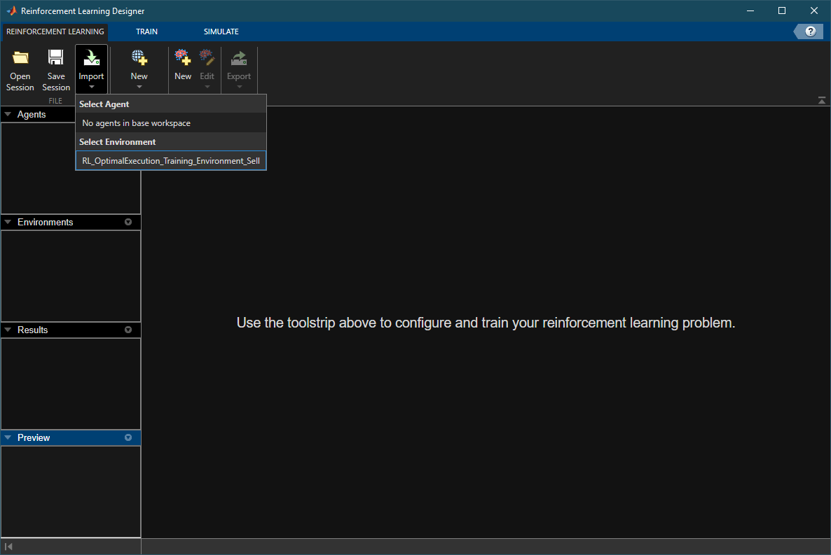
Open Reinforcement Learning Designer (Reinforcement Learning Toolbox).
reinforcementLearningDesigner
Import the training environment by clicking the Import button and selecting the created training environment.
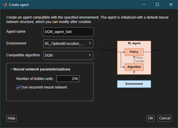
Create a new DQN agent by selecting New > Agent, then selecting DQN from the Compatible algorithm menu. Enable LSTM by selecting Use recurrent neural network.
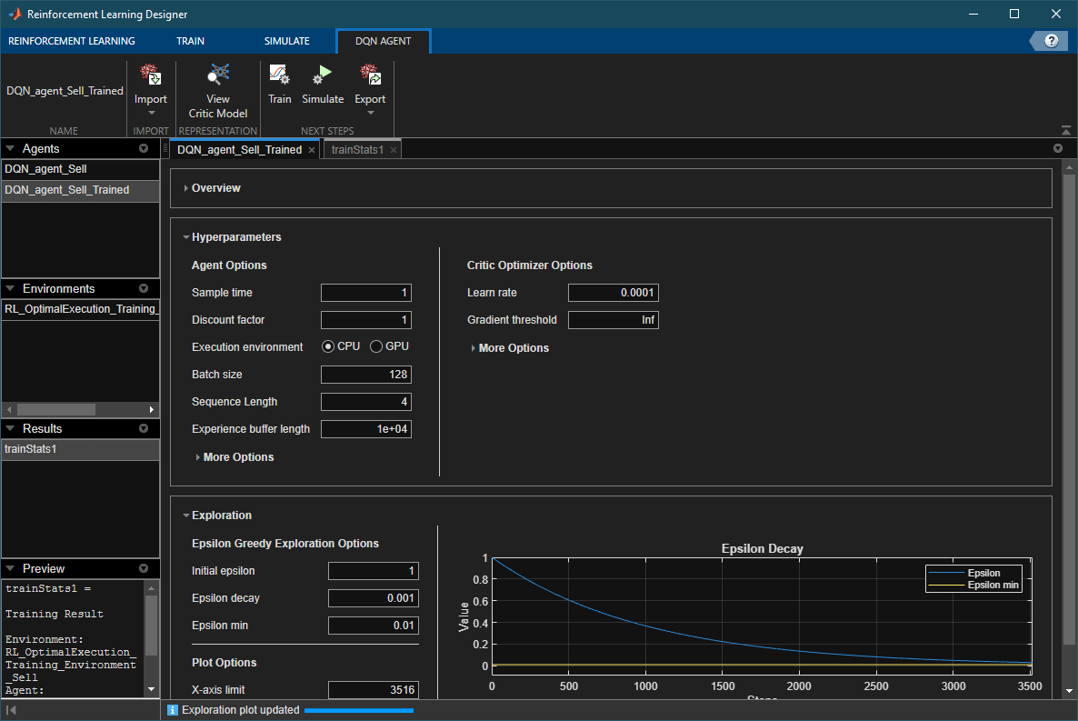
Set the agent hyperparameters and exploration parameters in the DQN Agent tab. Use the default options, except for the following:
Discount factor —
1Learn rate —
0.0001Batch size —
128Sequence length —
4Initial epsilon —
1Epsilon decay —
0.001
Go to the Train tab, and set the Max Episode Length to 3516 (NumTrainingSteps). You can experiment with different Stopping Criteria, or you can manually stop the training by clicking on the Stop button. In this example, you set the Stopping Criteria to EpisodeCount and the Max Episodes to a value greater than or equal to EpisodeCount. Click Train to start the training.
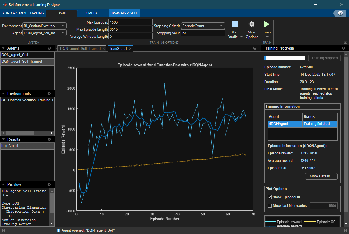
Once the training is complete, export the trained agent to the workspace. Since training can take a long time, you can load a pretrained agent (DQN_agent_Sell_Trained.mat) for sell trades.
load DQN_agent_Sell_Trained.matYou can view the DQN agent options by examining the AgentOptions property.
DQN_agent_Sell_Trained.AgentOptions
ans =
  rlDQNAgentOptions with properties:

                             SampleTime: 1
                         DiscountFactor: 1
               EpsilonGreedyExploration: [1×1 rl.option.EpsilonGreedyExploration]
                 ExperienceBufferLength: 10000
                          MiniBatchSize: 128
                         SequenceLength: 4
                 CriticOptimizerOptions: [1×1 rl.option.rlOptimizerOptions]
                    NumStepsToLookAhead: 1
                      NumWarmStartSteps: 128
                               NumEpoch: 1
                   MaxMiniBatchPerEpoch: 100
                      LearningFrequency: -1
                           UseDoubleDQN: 1
                     TargetSmoothFactor: 1.0000e-03
                  TargetUpdateFrequency: 1
            BatchDataRegularizerOptions: []
    ResetExperienceBufferBeforeTraining: 0
                             InfoToSave: [1×1 struct]
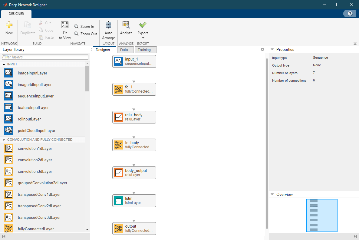
Also, you can visualize the DQN agent's critic network by using Deep Network Designer (Deep Learning Toolbox).
deepNetworkDesigner(layerGraph(getModel(getCritic(DQN_agent_Sell_Trained))))
Compute IS Using Trained Agent and Training Data for Sell Trades
Simulate selling actions using the trained agent and training environment.
rng('default');
reset(RL_OptimalExecution_Training_Environment_Sell);
Reset!
simOptions = rlSimulationOptions(MaxSteps=NumTrainingSteps)
simOptions =
  rlSimulationOptions with properties:

                   MaxSteps: 3516
             NumSimulations: 1
                StopOnError: "on"
      SimulationStorageType: "memory"
    SaveSimulationDirectory: "savedSims"
            SaveFileVersion: "-v7"
                UseParallel: 0
     ParallelizationOptions: [1×1 rl.option.ParallelSimulation]
Trained_Agent_Sell = DQN_agent_Sell_Trained;
experience_Sell = sim(RL_OptimalExecution_Training_Environment_Sell,Trained_Agent_Sell,simOptions);
Reset!
Last Horizon. Episode is Done!
HorizonIdx:
ans =
293
SimAction_Train_Sell = squeeze(experience_Sell.Action.TradingAction_NumberOfShares_.Data);
Compute the IS using simulated actions on the training data.
NumSimSteps = length(SimAction_Train_Sell);
SimInventory_Train_Sell = nan(NumSimSteps,1);
SimExecutedShares_Train_Sell = SimInventory_Train_Sell;
SimReward_Train_Sell = nan(NumSimSteps,1);

reset(RL_OptimalExecution_Training_Environment_Sell);
Reset!
for k=1:NumSimSteps
    [~,SimReward_Train_Sell(k),~,LoggedSignals] = ...
        step(RL_OptimalExecution_Training_Environment_Sell,SimAction_Train_Sell(k));
    SimInventory_Train_Sell(k) = LoggedSignals.CurrentInventoryShares;
    SimExecutedShares_Train_Sell(k) = sum(LoggedSignals.ExecutedShares);
end
Last Horizon. Episode is Done!
HorizonIdx:
ans =
293
IS_Agent_Step_Train_Sell = LoggedSignals.IS_Agent;
IS_Agent_Horizon_Train_Sell = IS_Agent_Step_Train_Sell( ....
    NumIntervalsPerHorizon:NumIntervalsPerHorizon:NumTrainingSteps);
Plot Training Results for Sell Trades
Plot Implementation Shortfall (IS), executed shares, and inventory shares for the agent for each step using training data.
figure
subplot(3,1,1)
bar(1:NumTrainingSteps, IS_Agent_Step_Train_Sell)
xlabel(strcat("Step number (", num2str(TradingIntervalSec), ...
    " sec intervals, ", num2str(NumTrainingSteps), " steps total.)"))
ylabel("Implementation Shortfall")
title("Implementation Shortfall  (Agent, Training, Sell)")
xlim([0 300])
ylim([-200 200])

subplot(3,1,2)
bar(1:NumTrainingSteps, SimExecutedShares_Train_Sell)
xlabel(strcat("Step number (", num2str(TradingIntervalSec), ...
    " sec intervals, ", num2str(NumTrainingSteps), " steps total.)"))
ylabel("Executed Shares")
title("Shares Traded at Each Step (Agent, Training, Sell)")
xlim([0 300])

subplot(3,1,3)
bar(1:NumTrainingSteps, SimInventory_Train_Sell)
xlabel(strcat("Step number (", num2str(TradingIntervalSec), ...
    " sec intervals, ", num2str(NumTrainingSteps), " steps total.)"))
ylabel("Inventory Shares")
title("Inventory Shares (Agent, Training, Sell)")
xlim([0 300])
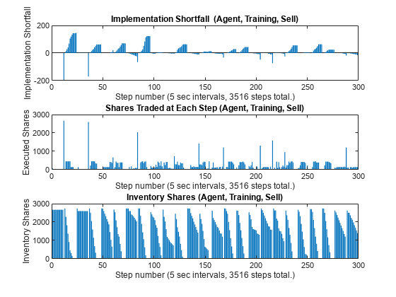
Unlike the previous TWAP baseline plot, where the executed shares in the middle panel have a flat profile, here you can see that the agent actively changes the number of executed shares at each step. Also, the inventory shares in the bottom panel decline in a non-linear manner.
To directly compare the results from the agent with the TWAP baseline, you can plot both results on the same chart. Generate plots to compare implementation shortfall, executed shares, and inventory shares between the TWAP baseline and the agent for each step using the training data.
figure
subplot(3,1,1)
plot(1:NumTrainingSteps, [IS_TWAP_Step_Train_Sell IS_Agent_Step_Train_Sell], linewidth=1.5)
xlabel(strcat("Step number (", num2str(TradingIntervalSec), ...
    " sec intervals, ", num2str(NumTrainingSteps), " steps total.)"))
ylabel("Implementation Shortfall")
title("Implementation Shortfall (Training, Sell)")
legend(["TWAP" "Agent"], location="east")
xlim([0 300])

subplot(3,1,2)
plot(1:NumTrainingSteps, [TradingShares_Step_TWAP_Train_Sell ...
    SimExecutedShares_Train_Sell], linewidth=1.5)
xlabel(strcat("Step number (", num2str(TradingIntervalSec), ...
    " sec intervals, ", num2str(NumTrainingSteps), " steps total.)"))
ylabel("Executed Shares")
title("Shares Traded at Each Step (Training, Sell)")
legend(["TWAP" "Agent"], location="east")
xlim([0 300])

subplot(3,1,3)
plot(1:NumTrainingSteps, [InventoryShares_Step_TWAP_Train_Sell ...
    SimInventory_Train_Sell], linewidth=1.5)
xlabel(strcat("Step number (", num2str(TradingIntervalSec), ...
    " sec intervals, ", num2str(NumTrainingSteps), " steps total.)"))
ylabel("Inventory Shares")
title("Inventory Shares (Training, Sell)")
legend(["TWAP" "Agent"], location="east")
xlim([0 300])

You can see the differences between the TWAP baseline (blue) and the agent (red) in their IS, executed shares, and inventory shares. Also, the agent tends to behave differently when the IS trends negative as compared to positive.
For example, in the first horizon (step numbers 1 to 12) and the third horizon (step numbers 25 to 36), the IS trends negative (more favorable prices than the arrival price) and the agent initially trades fewer shares than TWAP, until there are large spikes in the executed shares at the ends of the horizons to meet the ending inventory constraint. Also, the inventories initially declines more slowly than TWAP, until the abrupt declines to zero at the end of the horizon. This coincided with negative pulls in the agent's IS at the end of the first and the third horizons that go even lower than the IS of TWAP.
On the other hand, in the second horizon (step numbers 13 to 24), the IS trends positive (less favorable prices than the arrival price), and the agent initially trades more shares than TWAP to liquidate the inventory faster than TWAP. This has a limiting effect on the agent's IS at the end of the horizon, which is also lower than the IS of TWAP.
You can see similar behaviors in other horizons, although they do not always lead to an outperformance of the agent over TWAP.
Also, you can plot the differences in IS between TWAP and the agent, and then compare them with the rewards.
figure
subplot(3,1,1)
bar(1:NumTrainingHorizons, IS_TWAP_Horizon_Train_Sell - IS_Agent_Horizon_Train_Sell)
xlabel(strcat("Horizon number (", num2str(NumTrainingHorizons), " horizons total.)"))
title("IS TWAP - IS Agent Over Horizon (Training, Sell)")
xlim([0 43])
subplot(3,1,2)
bar(1:NumTrainingSteps, IS_TWAP_Step_Train_Sell - IS_Agent_Step_Train_Sell)
xlabel(strcat("Step number (", num2str(TradingIntervalSec), ...
    " sec intervals, ", num2str(NumTrainingSteps), " steps total.)"))
title("IS TWAP - IS Agent Each Step (Training, Sell)")
xlim([0 510])
subplot(3,1,3)
bar(1:NumTrainingSteps, SimReward_Train_Sell)
xlabel(strcat("Step number (", num2str(TradingIntervalSec), ...
    " sec intervals, ", num2str(NumTrainingSteps), " steps total.)"))
title("Reward (Training, Sell)")
xlim([0 510])
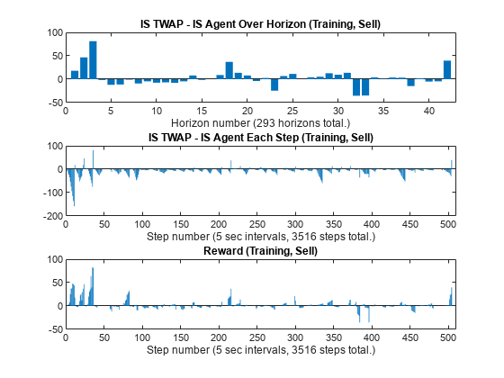
The top panel () shows the final performance of the agent for the training data as the differences in IS between TWAP and the agent at the ends of the horizons at times . For example, in the top panel, you can see the outperformance of the agent (positive IS difference) in the first three horizons, while the agent underperforms in some of the other horizons. The middle panel () shows the differences in IS for all time steps , including the ones before the ends of the horizons. The middle panel does not appear to track the top panel values very well in some steps (except for the very last steps in the horizons, which are the top panel values when ), as there are frequent trend reversals between negative and positive values at the last steps of the horizons. Therefore, the simple difference in IS between TWAP and the agent at each step () shown in the middle panel may not be a good reward function. On the other hand, the bottom panel, which plots the rewards used by the agent in this example at each step, appears to track the top panel values more closely than the middle panel at most steps.
Display Summary of Training Results for Sell Trades
Display the total Implementation Shortfall outperformance of the agent over TWAP for the training data.
sum(IS_TWAP_Horizon_Train_Sell - IS_Agent_Horizon_Train_Sell)
ans =
164.4700
Display total-gain-to-loss ratio (TGLR) for the training data.
ISTGLR(IS_TWAP_Horizon_Train_Sell - IS_Agent_Horizon_Train_Sell)
ans =
1.2327
TWAP Baseline Analysis on Testing Data
Using the same trained agent as the Compute IS Using Trained Agent and Training Data for Sell Trades section, you can perform the same analysis on the testing data that you kept separate from the training data.
First, execute the TWAP trades and compute IS for the testing data.
[IS_TWAP_Horizon_Test_Sell,IS_TWAP_Step_Test_Sell, ...
    InventoryShares_Step_TWAP_Test_Sell,TradingShares_Step_TWAP_Test_Sell] = ...
    executeTWAPTrades(TestingLOB,NumLevels,TotalTradingShares_Sell,...
    NumIntervalsPerHorizon,NumTestingHorizons,BuyTrade);
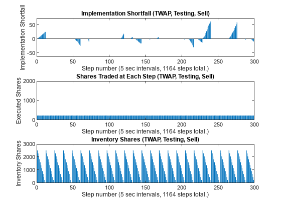
Plot the implementation shortfall, executed shares, and inventory shares for the TWAP baseline for each step using testing data.
figure
subplot(3,1,1)
bar(1:NumTestingSteps, IS_TWAP_Step_Test_Sell)
xlabel(strcat("Step number (", num2str(TradingIntervalSec), ...
    " sec intervals, ", num2str(NumTestingSteps), " steps total.)"))
ylabel("Implementation Shortfall")
title("Implementation Shortfall (TWAP, Testing, Sell)")
xlim([0 300])
ylim([-65 75])

subplot(3,1,2)
bar(1:NumTestingSteps, TradingShares_Step_TWAP_Test_Sell)
xlabel(strcat("Step number (", num2str(TradingIntervalSec), ...
    " sec intervals, ", num2str(NumTestingSteps), " steps total.)"))
ylabel("Executed Shares")
title("Shares Traded at Each Step (TWAP, Testing, Sell)")
xlim([0 300])
ylim([0 2000])

subplot(3,1,3)
bar(1:NumTestingSteps, InventoryShares_Step_TWAP_Test_Sell)
xlabel(strcat("Step number (", num2str(TradingIntervalSec), ...
    " sec intervals, ", num2str(NumTestingSteps), " steps total.)"))
ylabel("Inventory Shares")
title("Inventory Shares (TWAP, Testing, Sell)")
xlim([0 300])
Set Up RL Testing Environment for Sell Trades
Next, define the reset function for the testing environment.
EnvConstants_Test_Sell.SampledBook = TestingLOB;
EnvConstants_Test_Sell.BuyTrade = BuyTrade;
EnvConstants_Test_Sell.TotalTradingShares = TotalTradingShares_Sell;
EnvConstants_Test_Sell.NumIntervalsPerHorizon = NumIntervalsPerHorizon;
EnvConstants_Test_Sell.NumHorizons = NumTestingHorizons;
EnvConstants_Test_Sell.NumSteps = NumTestingSteps;
EnvConstants_Test_Sell.NumLevels = NumLevels;
EnvConstants_Test_Sell.IS_TWAP = IS_TWAP_Step_Test_Sell;

ResetFunction_Test_Sell = @() RL_OptimalExecution_LOB_ResetFcn(EnvConstants_Test_Sell);
Define the step function for the testing environment.
StepFunction_Test_Sell = @(Action,LoggedSignals) ...
    RL_OptimalExecution_LOB_StepFcn(Action,LoggedSignals,EnvConstants_Test_Sell);
Create the testing environment using the reset and step function handles.
RL_OptimalExecution_Testing_Environment_Sell = ...
    rlFunctionEnv(ObservationInfo_Train_Sell,ActionInfo_Sell, ...
    StepFunction_Test_Sell,ResetFunction_Test_Sell)
Reset!
Reset!
RL_OptimalExecution_Testing_Environment_Sell =
  rlFunctionEnv with properties:

     StepFcn: @(Action,LoggedSignals)RL_OptimalExecution_LOB_StepFcn(Action,LoggedSignals,EnvConstants_Test_Sell)
    ResetFcn: @()RL_OptimalExecution_LOB_ResetFcn(EnvConstants_Test_Sell)
        Info: [1×1 struct]
Validate Testing Environment Reset and Step Functions for Sell Trades
Now, validate the testing environment using reset and step function handles.
InitialObservation = reset(RL_OptimalExecution_Testing_Environment_Sell);
Reset!
InitialObservation
InitialObservation = 1×4

    2738    12    0    0
[~,Reward1,~,LoggedSignals1] = step( ...
    RL_OptimalExecution_Testing_Environment_Sell,TradingShares_Step_TWAP_Train_Sell(1));
LoggedSignals1
LoggedSignals1 = struct with fields:
IntervalIdx: 1
HorizonIdx: 1
CurrentInventoryShares: 2624
ArrivalPrice: 26.8000
ExecutedShares: 114
ExecutedPrices: 26.8000
HorizonExecutedShares: [60×1 double]
HorizonExecutedPrices: [60×1 double]
IS_Agent: [1164×1 double]
Reward: [1164×1 double]
NumIntervalsPerHorizon: 12
NumHorizons: 97
NumLevels: 5
Reward1
Reward1 =
0
[~,Reward2,~,LoggedSignals2] = step( ...
    RL_OptimalExecution_Testing_Environment_Sell,10);
LoggedSignals2
LoggedSignals2 = struct with fields:
IntervalIdx: 2
HorizonIdx: 1
CurrentInventoryShares: 2614
ArrivalPrice: 26.8000
ExecutedShares: 10
ExecutedPrices: 26.7900
HorizonExecutedShares: [60×1 double]
HorizonExecutedPrices: [60×1 double]
IS_Agent: [1164×1 double]
Reward: [1164×1 double]
NumIntervalsPerHorizon: 12
NumHorizons: 97
NumLevels: 5
Reward2
Reward2 =
-0.2050
[~,Reward3,~,LoggedSignals3] = step( ...
    RL_OptimalExecution_Testing_Environment_Sell,35);
LoggedSignals3
LoggedSignals3 = struct with fields:
IntervalIdx: 3
HorizonIdx: 1
CurrentInventoryShares: 2579
ArrivalPrice: 26.8000
ExecutedShares: 35
ExecutedPrices: 26.7900
HorizonExecutedShares: [60×1 double]
HorizonExecutedPrices: [60×1 double]
IS_Agent: [1164×1 double]
Reward: [1164×1 double]
NumIntervalsPerHorizon: 12
NumHorizons: 97
NumLevels: 5
Reward3
Reward3 =
-0.2975
Call the reset function again to restore the environment back to the initial state.
reset(RL_OptimalExecution_Testing_Environment_Sell);
Reset!
Compute IS Using Trained Agent and Testing Data for Sell Trades
Simulate actions using the trained agent and testing data for sell trades.
simOptions = rlSimulationOptions(MaxSteps=NumTestingSteps);
experience_Sell = sim(RL_OptimalExecution_Testing_Environment_Sell,Trained_Agent_Sell,simOptions);
Reset!
Last Horizon. Episode is Done!
HorizonIdx:
ans =
97
SimAction_Test_Sell = squeeze(experience_Sell.Action.TradingAction_NumberOfShares_.Data);
Compute Implementation Shortfall (IS) using simulated actions on testing data.
NumSimSteps = length(SimAction_Test_Sell);
SimInventory_Test_Sell = nan(NumSimSteps,1);
SimExecutedShares_Test_Sell = SimInventory_Test_Sell;
SimReward_Test_Sell = nan(NumSimSteps,1);

reset(RL_OptimalExecution_Testing_Environment_Sell);
Reset!
for k=1:NumSimSteps
    [~,SimReward_Test_Sell(k),~,LoggedSignals] = step( ...
        RL_OptimalExecution_Testing_Environment_Sell,SimAction_Test_Sell(k));
    SimInventory_Test_Sell(k) = LoggedSignals.CurrentInventoryShares;
    SimExecutedShares_Test_Sell(k) = sum(LoggedSignals.ExecutedShares);
end
Last Horizon. Episode is Done!
HorizonIdx:
ans =
97
IS_Agent_Step_Test_Sell = LoggedSignals.IS_Agent;
IS_Agent_Horizon_Test_Sell = IS_Agent_Step_Test_Sell( ...
    NumIntervalsPerHorizon:NumIntervalsPerHorizon:NumTestingSteps);
Plot Testing Results for Sell Trades
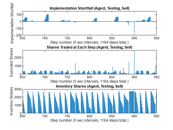
Plot Implementation Shortfall (IS), executed shares, and inventory shares of the agent for each step using testing data.
figure
subplot(3,1,1)
bar(1:NumTestingSteps, IS_Agent_Step_Test_Sell)
xlabel(strcat("Step number (", num2str(TradingIntervalSec), ...
    " sec intervals, ", num2str(NumTestingSteps), " steps total.)"))
ylabel("Implementation Shortfall")
title("Implementation Shortfall (Agent, Testing, Sell)")
xlim([650 950])
ylim([-200 150])

subplot(3,1,2)
bar(1:NumTestingSteps, SimExecutedShares_Test_Sell)
xlabel(strcat("Step number (", num2str(TradingIntervalSec), ...
    " sec intervals, ", num2str(NumTestingSteps), " steps total.)"))
ylabel("Executed Shares")
title("Shares Traded at Each Step (Agent, Testing, Sell)")
xlim([650 950])
ylim([0 2900])

subplot(3,1,3)
bar(1:NumTestingSteps, SimInventory_Test_Sell)
xlabel(strcat("Step number (", num2str(TradingIntervalSec), ...
    " sec intervals, ", num2str(NumTestingSteps), " steps total.)"))
ylabel("Inventory Shares")
title("Inventory Shares (Agent, Testing, Sell)")
xlim([650 950])
Compare implementation shortfall, executed shares, and inventory shares between the TWAP baseline and the agent for each step using testing data.
figure
subplot(3,1,1)
plot(1:NumTestingSteps, [IS_TWAP_Step_Test_Sell IS_Agent_Step_Test_Sell], linewidth=1.5)
xlabel(strcat("Step number (", num2str(TradingIntervalSec), ...
    " sec intervals, ", num2str(NumTestingSteps), " steps total.)"))
ylabel("Implementation Shortfall")
title("Implementation Shortfall (Testing, Sell)")
legend(["TWAP" "Agent"],location='best')
xlim([650 950])
ylim([-200 150])

subplot(3,1,2)
plot(1:NumTestingSteps, [TradingShares_Step_TWAP_Test_Sell ...
    SimExecutedShares_Test_Sell], linewidth=1.5)
xlabel(strcat("Step number (", num2str(TradingIntervalSec), ...
    " sec intervals, ", num2str(NumTestingSteps), " steps total.)"))
ylabel("Executed Shares")
title("Shares Traded at Each Step (Testing, Sell)")
legend(["TWAP" "Agent"])
xlim([650 950])
ylim([0 2900])

subplot(3,1,3)
plot(1:NumTestingSteps, [InventoryShares_Step_TWAP_Test_Sell ...
    SimInventory_Test_Sell], linewidth=1.5)
xlabel(strcat("Step number (", num2str(TradingIntervalSec), ...
    " sec intervals, ", num2str(NumTestingSteps), " steps total.)"))
ylabel("Inventory Shares")
title("Inventory Shares (Testing, Sell)")
legend(["TWAP" "Agent"])
xlim([650 950])
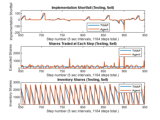
Just as in the training data, the agent (red) actively changes the number of executed shares for each step in the testing data, while the TWAP policy (blue) executes the same number of shares at each step.
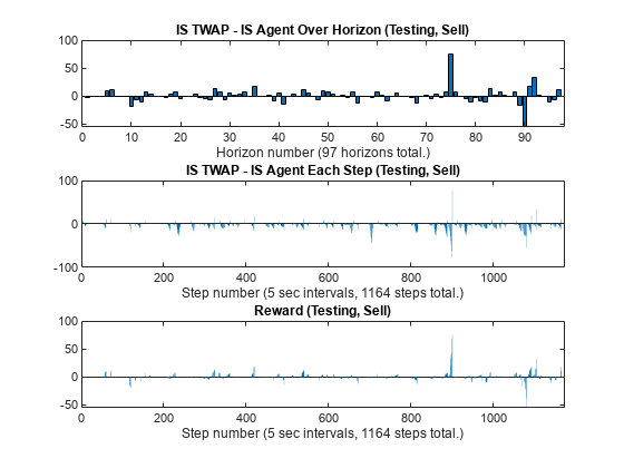
Plot the differences in IS between TWAP and the agent and then compare them with the rewards.
figure
subplot(3,1,1)
bar(1:NumTestingHorizons, IS_TWAP_Horizon_Test_Sell - IS_Agent_Horizon_Test_Sell)
xlabel(strcat("Horizon number (", num2str(NumTestingHorizons), " horizons total.)"))
title("IS TWAP - IS Agent Over Horizon (Testing, Sell)")

subplot(3,1,2)
bar(1:NumTestingSteps, IS_TWAP_Step_Test_Sell - IS_Agent_Step_Test_Sell)
xlabel(strcat("Step number (", num2str(TradingIntervalSec), ...
    " sec intervals, ", num2str(NumTestingSteps), " steps total.)"))
title("IS TWAP - IS Agent Each Step (Testing, Sell)")
xlim([0 NumTestingSteps+9])

subplot(3,1,3)
bar(1:NumTestingSteps, SimReward_Test_Sell)
xlabel(strcat("Step number (", num2str(TradingIntervalSec), ...
    " sec intervals, ", num2str(NumTestingSteps), " steps total.)"))
title("Reward (Testing, Sell)")
xlim([0 NumTestingSteps+9])
Display Summary of Training and Testing Results for Sell Trades
You can summarize the results of the sell trade agent's training and testing.
Display total Implementation Shortfall (IS) outperformance of the agent over TWAP for training data.
Total_Outperformance_Train_Sell = sum(IS_TWAP_Horizon_Train_Sell - IS_Agent_Horizon_Train_Sell);
table(Total_Outperformance_Train_Sell)
ans=table
    Total_Outperformance_Train_Sell
    _______________________________

                164.47
Display total-gain-to-loss ratio (TGLR) and gain-to-loss ratio (GLR) for the training data.
[TGLR_Train_Sell, GLR_Train_Sell] = ...
    ISTGLR(IS_TWAP_Horizon_Train_Sell - IS_Agent_Horizon_Train_Sell);

table(TGLR_Train_Sell, GLR_Train_Sell)ans=1×2 table
TGLR_Train_Sell GLR_Train_Sell
_______________ ______________
1.2327 1.2532
Display the total IS outperformance of the agent over TWAP for the testing data.
Total_Outperformance_Test_Sell = sum(IS_TWAP_Horizon_Test_Sell - IS_Agent_Horizon_Test_Sell);
table(Total_Outperformance_Test_Sell)
ans=table
    Total_Outperformance_Test_Sell
    ______________________________

                104.12
Display TGLR and GLR for the testing data.
[TGLR_Test_Sell, GLR_Test_Sell] = ...
    ISTGLR(IS_TWAP_Horizon_Test_Sell - IS_Agent_Horizon_Test_Sell);
table(TGLR_Test_Sell, GLR_Test_Sell)ans=1×2 table
TGLR_Test_Sell GLR_Test_Sell
______________ _____________
1.389 1.1906
Optimal Execution for Buy Trades
You can use a shortened version of the previous procedure (Optimal Execution for Sell Trades) to support the workflow for designing a DQN agent for optimal execution of buy trades. To repeat the same workflow for buy trades, first set the BuyTrade logical flag to true and define the total number of shares to buy over the horizon.
BuyTrade = true;
TotalTradingShares_Buy = 2551;
Execute TWAP trades and compute the Implementation Shortfall (IS).
[IS_TWAP_Horizon_Train_Buy,IS_TWAP_Step_Train_Buy, ...
    InventoryShares_Step_TWAP_Train_Buy,TradingShares_Step_TWAP_Train_Buy] = ...
    executeTWAPTrades(TrainingLOB,NumLevels,TotalTradingShares_Buy, ...
    NumIntervalsPerHorizon,NumTrainingHorizons,BuyTrade);
Set up the RL training environment for buy trades.
ObservationDimension = [1 4];
ObservationInfo_Train_Buy = rlNumericSpec(ObservationDimension);
ObservationInfo_Train_Buy.Name = 'Observation Data';
ObservationInfo_Train_Buy.Description = ['RemainingSharesToTrade, ...' ...
    'RemainingIntervals, IS_Agent, PriceDivergence'];
ObservationInfo_Train_Buy.LowerLimit = -inf;
ObservationInfo_Train_Buy.UpperLimit = inf;

EnvConstants_Train_Buy.SampledBook = TrainingLOB;
EnvConstants_Train_Buy.BuyTrade = BuyTrade;
EnvConstants_Train_Buy.TotalTradingShares = TotalTradingShares_Buy;
EnvConstants_Train_Buy.NumIntervalsPerHorizon = NumIntervalsPerHorizon;
EnvConstants_Train_Buy.NumHorizons = NumTrainingHorizons;
EnvConstants_Train_Buy.NumSteps = NumTrainingSteps;
EnvConstants_Train_Buy.NumLevels = NumLevels;
EnvConstants_Train_Buy.IS_TWAP = IS_TWAP_Step_Train_Buy;
ResetFunction_Buy = @() RL_OptimalExecution_LOB_ResetFcn(EnvConstants_Train_Buy);

NumActions = 39;
LowerActionRange = linspace(0,TradingShares_Step_TWAP_Train_Buy(1), round(NumActions/2));
ActionRange = round([LowerActionRange(1:end-1) ...
    linspace(TradingShares_Step_TWAP_Train_Buy(1), ...
    TradingShares_Step_TWAP_Train_Buy(1)*2,round(NumActions/2))]);
NumActions = length(ActionRange);

ActionInfo_Buy = rlFiniteSetSpec(ActionRange);
ActionInfo_Buy.Name = 'Trading Action (Number of Shares)';
ActionInfo_Buy.Description = 'Number of Shares to be Traded at Each Time Step';

StepFunction_Train_Buy = @(Action,LoggedSignals) ...
    RL_OptimalExecution_LOB_StepFcn(Action,LoggedSignals,EnvConstants_Train_Buy);

RL_OptimalExecution_Training_Environment_Buy = rlFunctionEnv( ...
    ObservationInfo_Train_Buy,ActionInfo_Buy,StepFunction_Train_Buy,ResetFunction_Buy)
Reset!
Reset!
RL_OptimalExecution_Training_Environment_Buy =
  rlFunctionEnv with properties:

     StepFcn: @(Action,LoggedSignals)RL_OptimalExecution_LOB_StepFcn(Action,LoggedSignals,EnvConstants_Train_Buy)
    ResetFcn: @()RL_OptimalExecution_LOB_ResetFcn(EnvConstants_Train_Buy)
        Info: [1×1 struct]
Use Reinforcement Learning Designer (Reinforcement Learning Toolbox) to create and train the agent for the buy trades. You use the same procedure (Optimal Execution for Sell Trades) as with the sell trades, except that the imported training environment is for buy trades (RL_OptimalExecution_Training_Environment_Buy). Once the training is complete, export the trained agent to the workspace. Since training can take a long time, this example uses a pretrained agent (DQN_agent_Buy_Trained.mat).
load DQN_agent_Buy_Trained.matCompute IS using the trained agent and training data for buy trades.
rng('default');
reset(RL_OptimalExecution_Training_Environment_Buy);
Reset!
simOptions = rlSimulationOptions(MaxSteps=NumTrainingSteps);
Trained_Agent_Buy = DQN_agent_Buy_Trained;
experience_Buy = sim(RL_OptimalExecution_Training_Environment_Buy,Trained_Agent_Buy,simOptions);
Reset!
Last Horizon. Episode is Done!
HorizonIdx:
ans =
293
SimAction_Train_Buy = squeeze(experience_Buy.Action.TradingAction_NumberOfShares_.Data);
NumSimSteps = length(SimAction_Train_Buy);
SimInventory_Train_Buy = nan(NumSimSteps,1);
SimExecutedShares_Train_Buy = SimInventory_Train_Buy;
SimReward_Train_Buy = nan(NumSimSteps,1);
reset(RL_OptimalExecution_Training_Environment_Buy);
Reset!
for k=1:NumSimSteps
    [~,SimReward_Train_Buy(k),~,LoggedSignals] = ...
        step(RL_OptimalExecution_Training_Environment_Buy,SimAction_Train_Buy(k));
    SimInventory_Train_Buy(k) = LoggedSignals.CurrentInventoryShares;
    SimExecutedShares_Train_Buy(k) = sum(LoggedSignals.ExecutedShares);
end
Last Horizon. Episode is Done!
HorizonIdx:
ans =
293
IS_Agent_Step_Train_Buy = LoggedSignals.IS_Agent;
IS_Agent_Horizon_Train_Buy = IS_Agent_Step_Train_Buy( ....
    NumIntervalsPerHorizon:NumIntervalsPerHorizon:NumTrainingSteps);
Execute the TWAP trades and compute the IS for the testing data.
[IS_TWAP_Horizon_Test_Buy,IS_TWAP_Step_Test_Buy, ...
    InventoryShares_Step_TWAP_Test_Buy,TradingShares_Step_TWAP_Test_Buy] = ...
    executeTWAPTrades(TestingLOB,NumLevels,TotalTradingShares_Buy, ...
    NumIntervalsPerHorizon,NumTestingHorizons,BuyTrade);
Set up the RL testing environment for buy trades.
EnvConstants_Test_Buy.SampledBook = TestingLOB;
EnvConstants_Test_Buy.BuyTrade = BuyTrade;
EnvConstants_Test_Buy.TotalTradingShares = TotalTradingShares_Buy;
EnvConstants_Test_Buy.NumIntervalsPerHorizon = NumIntervalsPerHorizon;
EnvConstants_Test_Buy.NumHorizons = NumTestingHorizons;
EnvConstants_Test_Buy.NumSteps = NumTestingSteps;
EnvConstants_Test_Buy.NumLevels = NumLevels;
EnvConstants_Test_Buy.IS_TWAP = IS_TWAP_Step_Test_Buy;
ResetFunction_Test_Buy = @() RL_OptimalExecution_LOB_ResetFcn(EnvConstants_Test_Buy);
StepFunction_Test_Buy = @(Action,LoggedSignals) ...
    RL_OptimalExecution_LOB_StepFcn(Action,LoggedSignals,EnvConstants_Test_Buy);
RL_OptimalExecution_Testing_Environment_Buy = ...
    rlFunctionEnv(ObservationInfo_Train_Buy,ActionInfo_Buy, ...
    StepFunction_Test_Buy,ResetFunction_Test_Buy)
Reset!
Reset!
RL_OptimalExecution_Testing_Environment_Buy =
  rlFunctionEnv with properties:

     StepFcn: @(Action,LoggedSignals)RL_OptimalExecution_LOB_StepFcn(Action,LoggedSignals,EnvConstants_Test_Buy)
    ResetFcn: @()RL_OptimalExecution_LOB_ResetFcn(EnvConstants_Test_Buy)
        Info: [1×1 struct]
Compute IS using the trained agent and testing data for buy trades.
simOptions = rlSimulationOptions(MaxSteps=NumTestingSteps);
experience_Buy = sim(RL_OptimalExecution_Testing_Environment_Buy,Trained_Agent_Buy,simOptions);
Reset!
Last Horizon. Episode is Done!
HorizonIdx:
ans =
97
SimAction_Test_Buy = squeeze(experience_Buy.Action.TradingAction_NumberOfShares_.Data);
NumSimSteps = length(SimAction_Test_Buy);
SimInventory_Test_Buy = nan(NumSimSteps,1);
SimExecutedShares_Test_Buy = SimInventory_Test_Buy;
SimReward_Test_Buy = nan(NumSimSteps,1);
reset(RL_OptimalExecution_Testing_Environment_Buy);
Reset!
for k=1:NumSimSteps
    [NextObs1,SimReward_Test_Buy(k),IsDone1,LoggedSignals] = step( ...
        RL_OptimalExecution_Testing_Environment_Buy,SimAction_Test_Buy(k));
    SimInventory_Test_Buy(k) = LoggedSignals.CurrentInventoryShares;
    SimExecutedShares_Test_Buy(k) = sum(LoggedSignals.ExecutedShares);
end
Last Horizon. Episode is Done!
HorizonIdx:
ans =
97
IS_Agent_Step_Test_Buy = LoggedSignals.IS_Agent;
IS_Agent_Horizon_Test_Buy = IS_Agent_Step_Test_Buy( ...
    NumIntervalsPerHorizon:NumIntervalsPerHorizon:NumTestingSteps);
Display the total Implementation Shortfall (IS) outperformance of the agent over TWAP for training data.
Total_Outperformance_Train_Buy = sum(IS_TWAP_Horizon_Train_Buy - IS_Agent_Horizon_Train_Buy);
table(Total_Outperformance_Train_Buy)
ans=table
    Total_Outperformance_Train_Buy
    ______________________________

                326.25
Display total-gain-to-loss ratio (TGLR) and gain-to-loss ratio (GLR) for the training data.
[TGLR_Train_Buy, GLR_Train_Buy] = ...
    ISTGLR(IS_TWAP_Horizon_Train_Buy - IS_Agent_Horizon_Train_Buy);
table(TGLR_Train_Buy, GLR_Train_Buy)ans=1×2 table
TGLR_Train_Buy GLR_Train_Buy
______________ _____________
1.4146 1.2587
Display total IS outperformance of the agent over TWAP for the testing data.
Total_Outperformance_Test_Buy = sum(IS_TWAP_Horizon_Test_Buy - IS_Agent_Horizon_Test_Buy);
table(Total_Outperformance_Test_Buy)
ans=table
    Total_Outperformance_Test_Buy
    _____________________________

               196.57
Display TGLR and GLR for the testing data.
[TGLR_Test_Buy, GLR_Test_Buy] = ...
    ISTGLR(IS_TWAP_Horizon_Test_Buy - IS_Agent_Horizon_Test_Buy);
table(TGLR_Test_Buy, GLR_Test_Buy)ans=1×2 table
TGLR_Test_Buy GLR_Test_Buy
_____________ ____________
2.018 1.4641
References
[1] Bertsimas, Dimitris, and Andrew W. Lo. "Optimal Control of Execution Costs." Journal of Financial Markets 1, no. 1 (1998): 1-50.
[2] Almgren, Robert, and Neil Chriss. "Optimal Execution of Portfolio Transactions." Journal of Risk 3, no. 2 (2000): 5-40.
[3] Nevmyvaka, Yuriy, Yi Feng, and Michael Kearns. "Reinforcement Learning for Optimized Trade Execution." In Proceedings of the 23rd International Conference on Machine Learning, pp. 673-680. 2006.
[4] Ning B., F. Lin, and S. Jaimungal. "Double Deep Q-Learning for Optimal Execution." Preprint, submitted June 8, 2020. Available at https://arxiv.org/abs/1812.06600.
[5] Lin S. and P. A. Beling. "Optimal Liquidation with Deep Reinforcement Learning." 33rd Conference on Neural Information Processing Systems (NeurIPS 2019) Deep Reinforcement Learning Workshop. Vancouver, Canada, 2019.
[6] Lin S. and P. A. Beling. "An End-to-End Optimal Trade Execution Framework Based on Proximal Policy Optimization." Proceedings of the 29th International Joint Conference on Artificial Intelligence (IJCAI 2020) Special Track on AI in FinTech. 4548-4554. 2020.
[7] LOBSTER Limit Order Book Data. Berlin: frischedaten UG (haftungsbeschränkt). Available at https://lobsterdata.com/home.
Local Functions
function [IS_TWAP_Horizon,IS_TWAP_Step,InventorySharesStepTWAP,TradingSharesStepTWAP] = ...
    executeTWAPTrades(InputLOB,NumLevels,TotalTradingShares,NumIntervalsPerHorizon,NumHorizons,BuyTrade)
% executeTWAPTrades Function for Executing Trades for TWAP Baseline
% This function executes buy or sell trades for the TWAP baseline and
% computes the corresponding implementation shortfalls, inventory shares
% and trading shares at each step.

NumSteps = NumHorizons*NumIntervalsPerHorizon;
IS_TWAP_Horizon = nan(NumHorizons,1);
IS_TWAP_Step = nan(NumSteps,1);
TradingSharesStepTWAP = round(TotalTradingShares./NumIntervalsPerHorizon).*ones(NumSteps,1);

if BuyTrade
    InventorySharesStepTWAP = zeros(NumSteps,1);
else
    InventorySharesStepTWAP = zeros(NumSteps,1) + TotalTradingShares;
end

for HorizonIdx = 1:NumHorizons
    HorizonExecutedPrices = zeros(NumLevels*NumIntervalsPerHorizon,1);
    HorizonExecutedShares = HorizonExecutedPrices;
    for IntervalIdx = 1:NumIntervalsPerHorizon
        CurrentBook =  InputLOB(IntervalIdx + NumIntervalsPerHorizon*(HorizonIdx-1),:);

        % Execute trade
        if IntervalIdx==NumIntervalsPerHorizon
            if BuyTrade
                % Enforce target ending inventory constraint for buy trade (buy missing shares)
                CurrentTradingShares = max(TotalTradingShares - ...
                    InventorySharesStepTWAP(IntervalIdx + NumIntervalsPerHorizon.*(HorizonIdx-1)), 0);
            else
                % Enforce zero ending inventory constraint for sell trade (sell remaining shares)
                CurrentTradingShares = max(InventorySharesStepTWAP(IntervalIdx + ...
                    NumIntervalsPerHorizon.*(HorizonIdx-1)), 0);
            end
        else
            CurrentTradingShares = TradingSharesStepTWAP(IntervalIdx + ...
                NumIntervalsPerHorizon.*(HorizonIdx-1));
        end

        [ExecutedShares,ExecutedPrices,InitialPrice,TradedLevels] = ...
            tradeLOB(CurrentBook,CurrentTradingShares,BuyTrade);
        if IntervalIdx==1
            ArrivalPrice = InitialPrice;
        end
        HorizonExecutedShares((1:TradedLevels) + (IntervalIdx-1)*NumLevels) = ExecutedShares;
        HorizonExecutedPrices((1:TradedLevels) + (IntervalIdx-1)*NumLevels) = ExecutedPrices;

        if BuyTrade
            InventorySharesStepTWAP((IntervalIdx:NumIntervalsPerHorizon) + ...
                NumIntervalsPerHorizon.*(HorizonIdx-1)) = ...
                InventorySharesStepTWAP(IntervalIdx + ...
                NumIntervalsPerHorizon.*(HorizonIdx-1)) + sum(ExecutedShares);
        else
            InventorySharesStepTWAP((IntervalIdx:NumIntervalsPerHorizon) + ...
                NumIntervalsPerHorizon.*(HorizonIdx-1)) = ...
                InventorySharesStepTWAP(IntervalIdx + ...
                NumIntervalsPerHorizon.*(HorizonIdx-1)) - sum(ExecutedShares);
        end

        % Compute Implementation Shortfall for each Step
        IS_TWAP_Step(IntervalIdx + NumIntervalsPerHorizon.*(HorizonIdx-1)) = ...
            endingInventoryIS(ArrivalPrice,HorizonExecutedPrices,HorizonExecutedShares,BuyTrade);
    end

    % Compute Implementation Shortfall for each Horizon
    IS_TWAP_Horizon(HorizonIdx) = endingInventoryIS(ArrivalPrice, ...
        HorizonExecutedPrices,HorizonExecutedShares,BuyTrade);
end

end


function [InitialObservation,LoggedSignals] = RL_OptimalExecution_LOB_ResetFcn(EnvConstants)
% RL_OptimalExecution_LOB_ResetFcn is Reset Function for RL Agent
% Define Reset Function
%
% Inputs:
%
% EnvConstants: Structure with the following fields:
% - SampledBook: Limit order book sampled at time intervals
% - BuyTrade: Scalar logical indicating the trading direction
%               true: Buy
%               false: Sell
% - TotalTradingShares: Number of shares to trade over the horizon (scalar)
% - NumIntervalsPerHorizon: Number of intervals per horizon (scalar)
% - NumHorizons: Number of horizons in the data (scalar)
% - NumSteps: Number of steps in the data (scalar)
% - NumLevels: Number of levels in the limit order book (scalar)
% - IS_TWAP: Implementation shortfall for TWAP baseline (NumSteps-by-1 vector)
%
% Outputs:
%
% InitialObservation:
% - Remaining shares to be traded by agent
% - Remaining intervals (steps) in the current trading horizon
% - Implementation shortfall of agent
% - Price divergence times 100
%
% LoggedSignals: Structure with following fields:
% - IntervalIdx: Current time interval index (initial value: 0)
% - HorizonIdx: Current time horizon index (initial value: 0)
% - CurrentInventoryShares: Current number of shares in inventory
%    (Initial value: 0 for Buy trade)
%    (Initial value: TotalTradingShares for Sell trade)
% - ArrivalPrice: Arrival price at the beginning of horizon (initial value: 0)
% - ExecutedShares: Number of executed shares at each traded level (initial value: 0)
% - ExecutedPrices: Prices of executed shares at each traded level (initial value: 0)
% - HorizonExecutedShares: Executed shares at each level over the horizon
%     (Initial value: (NumLevels * NumIntervalsPerHorizon)-by-1 vector of zeros)
% - HorizonExecutedPrices: Prices of Executed shares at each level over the horizon
%     (Initial value: (NumLevels * NumIntervalsPerHorizon)-by-1 vector of zeros)
% - IS_Agent: Implementation shortfall history of agent
%     (Initial value: NumIntervals-by-1 vector of zeros)
% - Reward: Reward history of agent
%     (Initial value: NumIntervals-by-1 vector of zeros)
% - NumIntervalsPerHorizon: Number of intervals per horizon (fixed value: NumIntervalsPerHorizon)
% - NumHorizons: Number of horizons (fixed value: NumHorizon)
% - NumLevels: Number of levels in the limit order book (fixed value: NumLevels)

IntervalIdx = 0;
HorizonIdx = 0;

LoggedSignals.IntervalIdx = IntervalIdx;
LoggedSignals.HorizonIdx = HorizonIdx;

InitialObservation = ...
    [EnvConstants.TotalTradingShares EnvConstants.NumIntervalsPerHorizon 0 0];

if EnvConstants.BuyTrade
    LoggedSignals.CurrentInventoryShares = 0;
else
    LoggedSignals.CurrentInventoryShares = EnvConstants.TotalTradingShares;
end

LoggedSignals.ArrivalPrice = 0;
LoggedSignals.ExecutedShares = 0;
LoggedSignals.ExecutedPrices = 0;
LoggedSignals.HorizonExecutedShares = ...
    zeros(EnvConstants.NumLevels*EnvConstants.NumIntervalsPerHorizon,1);
LoggedSignals.HorizonExecutedPrices = LoggedSignals.HorizonExecutedShares;
LoggedSignals.IS_Agent = zeros(EnvConstants.NumSteps,1);
LoggedSignals.Reward = LoggedSignals.IS_Agent;
LoggedSignals.NumIntervalsPerHorizon = EnvConstants.NumIntervalsPerHorizon;
LoggedSignals.NumHorizons = EnvConstants.NumHorizons;
LoggedSignals.NumLevels = EnvConstants.NumLevels;

disp("Reset!")
end

function [Observation,Reward,IsDone,LoggedSignals] = ...
    RL_OptimalExecution_LOB_StepFcn(Action,LoggedSignals,EnvConstants)
% RL_OptimalExecution_LOB_StepFcn function is Step Function for RL Environment
%   Given current Action and LoggedSignals, update Observation, Reward, and
%   LoggedSignals, and indicate whether the episode is complete.
%
% Inputs:
%
% Action: Number of shares to be traded at the current step (scalar)
%
% LoggedSignals: Structure with following fields
% - IntervalIdx: Current time interval index
% - HorizonIdx: Current time horizon index
% - CurrentInventoryShares: Current number of shares in inventory
% - ArrivalPrice: Arrival price at the beginning of horizon
% - ExecutedShares: Number of executed shares at each traded level
% - ExecutedPrices: Prices of executed shares at each traded level
% - HorizonExecutedShares: Executed shares at each level over the horizon
%     ((NumLevels * NumIntervalsPerHorizon)-by-1 vector)
% - HorizonExecutedPrices: Prices of Executed shares at each level over the horizon
%     ((NumLevels * NumIntervalsPerHorizon)-by-1 vector)
% - IS_Agent: Implementation shortfall history of agent
%     (NumIntervals-by-1 vector)
% - Reward: Reward history of agent
%     (NumIntervals-by-1 vector)
% - NumIntervalsPerHorizon: Number of intervals per horizon (fixed value: NumIntervalsPerHorizon)
% - NumHorizons: Number of horizons (fixed value: NumHorizon)
% - NumLevels: Number of levels in the limit order book (fixed value: NumLevels)
%
% EnvConstants: Structure with the following fields
% - SampledBook: Limit order book sampled at time intervals
% - BuyTrade: Scalar logical indicating the trading direction
%               true: Buy
%               false: Sell
% - TotalTradingShares: Number of shares to trade over the horizon (scalar)
% - NumIntervalsPerHorizon: Number of intervals per horizon (scalar)
% - NumHorizons: Number of horizons in the data (scalar)
% - NumSteps: Number of steps in the data (scalar)
% - NumLevels: Number of levels in the limit order book (scalar)
% - IS_TWAP: Implementation shortfall for TWAP baseline (NumSteps-by-1 vector)
%
% Outputs:
%
% Observation:
% - Remaining shares to be traded by agent
% - Remaining intervals (steps) in the current trading horizon
% - Implementation shortfall of agent
% - Price divergence times 100
%
% Reward: Reward for current step
%
% IsDone: Logical indicating whether the current episode is complete
%
% LoggedSignals: Updated LoggedSignals

% Update LoggedSignals indices
if (LoggedSignals.IntervalIdx == 0) && (LoggedSignals.HorizonIdx == 0)
    LoggedSignals.IntervalIdx = 1;
    LoggedSignals.HorizonIdx = 1;
elseif (LoggedSignals.IntervalIdx >= LoggedSignals.NumIntervalsPerHorizon)
    LoggedSignals.IntervalIdx = 1;
    LoggedSignals.HorizonIdx = LoggedSignals.HorizonIdx + 1;
    LoggedSignals.HorizonExecutedShares = ...
        zeros(EnvConstants.NumLevels*EnvConstants.NumIntervalsPerHorizon,1);
    LoggedSignals.HorizonExecutedPrices = LoggedSignals.HorizonExecutedShares;
    if EnvConstants.BuyTrade
        LoggedSignals.CurrentInventoryShares = 0;
    else
        LoggedSignals.CurrentInventoryShares = EnvConstants.TotalTradingShares;
    end
else
    LoggedSignals.IntervalIdx = LoggedSignals.IntervalIdx + 1;
end

StepIdx = LoggedSignals.IntervalIdx + ...
    LoggedSignals.NumIntervalsPerHorizon.*(LoggedSignals.HorizonIdx-1);
RemainingIntervals = LoggedSignals.NumIntervalsPerHorizon - LoggedSignals.IntervalIdx + 1;
IS_TWAP = EnvConstants.IS_TWAP(StepIdx);


if EnvConstants.BuyTrade
    AvgPrice = mean(EnvConstants.SampledBook(StepIdx,[1 5]),2);
    PriceDivergence = LoggedSignals.ArrivalPrice - AvgPrice;
else
    AvgPrice = mean(EnvConstants.SampledBook(StepIdx,[3 7]),2);
    PriceDivergence = AvgPrice - LoggedSignals.ArrivalPrice;
end

% Enforce ending inventory constraint
if LoggedSignals.IntervalIdx >= LoggedSignals.NumIntervalsPerHorizon
    if EnvConstants.BuyTrade
        TradingShares = max(EnvConstants.TotalTradingShares - ...
            LoggedSignals.CurrentInventoryShares, 0);
    else
        TradingShares = LoggedSignals.CurrentInventoryShares;
    end
else
    if EnvConstants.BuyTrade
        if PriceDivergence > 0
            AgentRemainingSharestoTrade = max(EnvConstants.TotalTradingShares - ...
                LoggedSignals.CurrentInventoryShares,0);
            TradingShares = round(AgentRemainingSharestoTrade./RemainingIntervals./2);
            TradingShares = min(TradingShares,Action);
        else
            TradingShares = min(EnvConstants.TotalTradingShares - ...
                LoggedSignals.CurrentInventoryShares, Action);
        end
    else
        if PriceDivergence > 0
            AgentRemainingSharestoTrade = max(LoggedSignals.CurrentInventoryShares, 0);
            TradingShares = round(AgentRemainingSharestoTrade./RemainingIntervals./2);
            TradingShares = min(TradingShares,Action);
        else
            TradingShares = min(LoggedSignals.CurrentInventoryShares, Action);
        end
    end
end

% Update IsDone:
% Episode is complete (IsDone is true) when time step reaches the end of
% the trading data.
if (LoggedSignals.HorizonIdx >= LoggedSignals.NumHorizons) && ...
        (LoggedSignals.IntervalIdx >= LoggedSignals.NumIntervalsPerHorizon)
    IsDone = true;
    disp("Last Horizon. Episode is Done!");
    disp("HorizonIdx:");
    LoggedSignals.HorizonIdx
elseif (LoggedSignals.IntervalIdx >= LoggedSignals.NumIntervalsPerHorizon)
    IsDone = false;
    % disp("HorizonIdx:");
    % LoggedSignals.HorizonIdx
else
    IsDone = false;
end

% Execute trade
CurrentLOB = EnvConstants.SampledBook(LoggedSignals.IntervalIdx + ...
    LoggedSignals.NumIntervalsPerHorizon*(LoggedSignals.HorizonIdx-1),:);

[ExecutedShares,ExecutedPrices,InitialPrice,TradedLevels] = ...
    tradeLOB(CurrentLOB,TradingShares,EnvConstants.BuyTrade);

% Update Reward
if LoggedSignals.IntervalIdx==1
    LoggedSignals.ArrivalPrice = InitialPrice;
end

LoggedSignals.HorizonExecutedShares((1:TradedLevels) + ...
    (LoggedSignals.IntervalIdx-1)*LoggedSignals.NumLevels) = ExecutedShares;
LoggedSignals.HorizonExecutedPrices((1:TradedLevels) + ...
    (LoggedSignals.IntervalIdx-1)*LoggedSignals.NumLevels) = ExecutedPrices;


IS_Agent = endingInventoryIS(LoggedSignals.ArrivalPrice,LoggedSignals.HorizonExecutedPrices, ...
    LoggedSignals.HorizonExecutedShares,EnvConstants.BuyTrade);

if EnvConstants.BuyTrade
    AgentRemainingSharestoTrade = max(EnvConstants.TotalTradingShares - ...
        LoggedSignals.CurrentInventoryShares - sum(ExecutedShares),0);
else
    AgentRemainingSharestoTrade = max(LoggedSignals.CurrentInventoryShares - ...
        sum(ExecutedShares), 0);
end

[PenaltyAgentExecutedShares,PenaltyAgentExecutedPrices] = tradeLOB(CurrentLOB, ...
    round(AgentRemainingSharestoTrade./RemainingIntervals),EnvConstants.BuyTrade);

IS_Agent_Penalty = RemainingIntervals.*endingInventoryIS(LoggedSignals.ArrivalPrice, ...
    PenaltyAgentExecutedPrices,PenaltyAgentExecutedShares,EnvConstants.BuyTrade);

TWAPRemainingSharestoTrade = (EnvConstants.NumIntervalsPerHorizon - LoggedSignals.IntervalIdx)* ...
    EnvConstants.TotalTradingShares/EnvConstants.NumIntervalsPerHorizon;

[PenaltyTWAPExecutedShares,PenaltyTWAPExecutedPrices] = tradeLOB(CurrentLOB, ...
    round(TWAPRemainingSharestoTrade./RemainingIntervals),EnvConstants.BuyTrade);

IS_TWAP_Penalty = RemainingIntervals.*endingInventoryIS(LoggedSignals.ArrivalPrice, ...
    PenaltyTWAPExecutedPrices,PenaltyTWAPExecutedShares,EnvConstants.BuyTrade);

Reward = ((IS_TWAP + IS_TWAP_Penalty) - (IS_Agent + IS_Agent_Penalty)) .* ...
    LoggedSignals.IntervalIdx./ LoggedSignals.NumIntervalsPerHorizon;

% No reward if trading target already met
if EnvConstants.BuyTrade
    if LoggedSignals.CurrentInventoryShares >= EnvConstants.TotalTradingShares
        Reward = 0;
    end
else
    if LoggedSignals.CurrentInventoryShares <= 0
        Reward = 0;
    end
end

% Update LoggedSignals
LoggedSignals.ExecutedPrices = ExecutedPrices;
LoggedSignals.ExecutedShares = ExecutedShares;

if EnvConstants.BuyTrade
    LoggedSignals.CurrentInventoryShares = ...
        LoggedSignals.CurrentInventoryShares + sum(ExecutedShares);
else
    LoggedSignals.CurrentInventoryShares = ...
        max(LoggedSignals.CurrentInventoryShares - sum(ExecutedShares), 0);
end

% Update LoggedSignals.IS_Agent
LoggedSignals.IS_Agent(StepIdx) = IS_Agent;

% Update LoggedSignals.Reward
LoggedSignals.Reward(StepIdx) = Reward;

% Update Observation
if LoggedSignals.IntervalIdx == LoggedSignals.NumIntervalsPerHorizon
    Observation = ...
        [EnvConstants.TotalTradingShares RemainingIntervals-1 IS_Agent PriceDivergence*100];
else
    Observation = ...
        [AgentRemainingSharestoTrade RemainingIntervals-1 IS_Agent PriceDivergence*100];
end

end


function [ExecutedShares,ExecutedPrices,InitialPrice,TradedLevels] = ...
    tradeLOB(CurrentLOB,TradingShares,BuyTrade)
% tradeLOB function executes market order trade based on current limit order book.
%   This function computes the results of executing a market order trade
%   for a specified number of shares and trade direction (buy/sell) based on
%   the information available in the current snapshot of the limit order book.
%
%   Inputs:
%
%      CurrentLOB - 1-by-(NumLevels*4) vector of current limit order book information
%
%         e.g. For NumLevels==5, 1-by-20 vector with the following values:
%    [AskPrice1 AskSize1 BidPrice1 BidSize1 ... AskPrice5 AskSize5 BidPrice5 BidSize5]
%
%         e.g. For NumLevels==10, 1-by-40 vector with the following values:
%    [AskPrice1 AskSize1 BidPrice1 BidSize1 ... AskPrice10 AskSize10 BidPrice10 BidSize10]
%
%      TradingShares - Scalar number of shares to be traded
%
%      BuyTrade - Scalar logical indicating trading direction:
%                    true: Buy
%                    false: Sell
%
%    Outputs:
%      ExecutedShares - Vector of number of executed shares at each traded level
%      ExecutedPrices - Vector of number of executed prices at each traded level
%      InitialPrice - Scalar numeric initial price
%      TradedLevels - Scalar numeric traded levels

LOBLength = length(CurrentLOB);

% Separate Bid and Ask data
AskPriceIdx = (1:4:LOBLength);
AskSizeIdx = AskPriceIdx + 1;
BidPriceIdx = AskSizeIdx + 1;
BidSizeIdx = BidPriceIdx + 1;

AskPrices = CurrentLOB(AskPriceIdx)';
AskSizes = CurrentLOB(AskSizeIdx)';
BidPrices = CurrentLOB(BidPriceIdx)';
BidSizes = CurrentLOB(BidSizeIdx)';

if BuyTrade
    LOBPrices = AskPrices;
    LOBSizes = AskSizes;
else
    LOBPrices = BidPrices;
    LOBSizes = BidSizes;
end

InitialPrice = LOBPrices(1);

% Execute trade
CumulativeLOBSizes = cumsum(LOBSizes);
TradedLevels = sum(CumulativeLOBSizes <= TradingShares);
if TradedLevels < 1
    TradedLevels = 1;
elseif CumulativeLOBSizes(TradedLevels) < TradingShares
    TradedLevels = TradedLevels + 1;
end

ExecutedPrices = LOBPrices(1:TradedLevels);
ExecutedShares = LOBSizes(1:TradedLevels);
ExecutedShares(end) = ExecutedShares(end) - (sum(ExecutedShares) - TradingShares);
end


function outIS = endingInventoryIS(ArrivalPrice,ExecutedPrices,TradedVolumes,BuyTrade)
% EndingInventoryIS function for Implementation Shortfall given ending inventory constraints
%   This function computes the Implementation Shortfall (IS) under the
%   assumption of ending inventory constraints (i.e. no opportunity cost).
%
%   For a Sell trade, the constraint is to have zero ending inventory
%   assuming successful liquidation of all shares.
%
%   For a Buy trade, the constraint is to have full ending inventory
%   assuming successful purchase of all shares.
%
%   Inputs:
%
%      ArrivalPrice - Scalar price immediately before trade execution
%
%      ExecutedPrices - Vector of executed prices
%
%      TradedVolumes - Vector of executed trade volumes
%
%      BuyTrade - Scalar logical indicating trading direction:
%                    true: Buy
%                    false: Sell
%
%    Outputs:
%      outIS - Implementation shortfall

outIS = ArrivalPrice.*sum(TradedVolumes) - sum(ExecutedPrices.*TradedVolumes);

if BuyTrade
    outIS = -outIS;
end

end


function [TGLR, GLR] = ISTGLR(ISDiffValues)
% ISTGLR function for Total-Gain-to-Loss Ratio for Implementation Shortfalls (IS)
%   This function computes the Total-Gain-to-Loss Ratio (TGLR) and the
%   Gain-to-Loss Ratio (GLR) for a vector of values (IS_Baseline - IS_Agent)
%   where:
%     - IS_Baseline: Implementation shortfalls for baseline (e.g. TWAP)
%     - IS_Agent: Implementation shortfalls for agent
%
%   Input:
%     - ISDiffValues: Vector of IS difference values (IS_Baseline - IS_Agent)
%
%   Outputs:
%     - TGLR: Total-Gain-to-Loss Ratio computed as the ratio of
%             Total Positive over Total Negative magnitudes of IS difference
%     - GLR:  Gain-to-Loss Ratio computed as the ratio of
%             Mean Positive over Mean Negative magnitudes of IS difference

ISDiffValues = ISDiffValues(:);

ISGains = ISDiffValues(ISDiffValues>0);
ISLosses = ISDiffValues(ISDiffValues<0);

MeanGains = abs(mean(ISGains));
MeanLosses = abs(mean(ISLosses));

TGLR = sum(ISGains)./abs(sum(ISLosses));
GLR = MeanGains./MeanLosses;

end