waldtest

Wald test of model specification

Syntax

h = waldtest(r,R,EstCov)

h = waldtest(r,R,EstCov,alpha)

[h,pValue] = waldtest(___)

[h,pValue,stat,cValue] = waldtest(___)

Description

h = waldtest(r,R,EstCov) returns the rejection decision from conducting a Wald test of model specification using the input restriction function and its Jacobian, and the value of the unrestricted model covariance estimator, all evaluated at the unrestricted parameter estimates.

• If any input argument is a cell vector of length k > 1, then the other input arguments must be cell arrays of length k. waldtest(r,R,EstCov) treats each cell as a separate, independent test, and returns a vector of rejection decisions.

• If any input argument is a row vector, then the software returns output arguments as row vectors.

h = waldtest(r,R,EstCov,alpha) returns the rejection decision of the Wald test conducted at the input significance level.

[h,pValue] = waldtest(___) returns the p-value of the hypothesis test, using any of the input arguments in the previous syntaxes.

[h,pValue,stat,cValue] = waldtest(___) returns the test statistic and critical value of the hypothesis test.

Examples

Assess Model Specifications Using the Wald Test

Check for significant lag effects in a time series regression model.

Load the U.S. GDP data set. Convert the serial dates to datetimes.

load Data_GDP
dt = datetime(dates,ConvertFrom="datenum");

Plot the GDP against time.

figure
plot(dt,Data)

The series seems to increase exponentially.

Transform the data using the natural logarithm.

logGDP = log(Data);

logGDP is increasing in time, so assume that there is a significant lag 1 effect. To use the Wald test to check if there is a significant lag 2 effect, you need the:

• Estimated coefficients of the unrestricted model

• Restriction function evaluated at the unrestricted model coefficient values

• Jacobian of the restriction function evaluated at the unrestricted model coefficient values

• Estimated, unrestricted parameter covariance matrix.

The unrestricted model is

$$y_t={\beta }_0+{\beta }_1{y}_{t-1}+{\beta }_2{y}_{t-2}+{\epsilon }_t.$$

Estimate the coefficients of the unrestricted model.

LagLGDP = lagmatrix(logGDP,1:2);
UMdl = fitlm(table(LagLGDP(:,1),LagLGDP(:,2),logGDP));

UMdl is a fitted LinearModel model. It contains, among other things, the fitted coefficients of the unrestricted model.

The restriction is $${\beta }_2=0$$. Therefore, the restriction function (r) and Jacobian (R) are:

• $$r={\beta }_2$$

• $$R=\left[\begin{array}{ccc}0& 0& 1\end{array}\right]$$

Specify r, R, and the estimated, unrestricted parameter covariance matrix.

r = UMdl.Coefficients.Estimate(3);
R = [0 0 1];
EstParamCov = UMdl.CoefficientCovariance;

Test for a significant lag 2 effect using the Wald test.

[h,pValue] = waldtest(r,R,EstParamCov)

h = logical
   1

pValue = 
1.2521e-07

h = 1 indicates that the null, restricted hypothesis ($${\beta }_2=0$$) should be rejected in favor of the alternative, unrestricted hypothesis. pValue is quite small, which suggests that there is strong evidence for this result.

Assess Conditional Heteroscedasticity Using the Wald Test

Test whether there are significant ARCH effects in a simulated response series using waldtest.

Suppose that the model for the simulated data is AR(1) with an ARCH(1) variance. Symbolically, the model is

$$y_t=0.9y_{t-1}+{\epsilon }_t,$$

where

• $${\epsilon }_t=w_t\sqrt{h_t}$$

• $$h_t=1+0.5{\epsilon }_{t-1}^2$$

• $$w_t$$ is Gaussian with mean 0 and variance 1.

Specify the model for the simulated data.

VarMdl = garch('ARCH',0.5,'Constant',1);
Mdl = arima('Constant',0,'Variance',VarMdl,'AR',0.9);

Mdl is a fully specified AR(1) model with an ARCH(1) variance.

Simulate presample and effective sample responses from Mdl.

T = 100;
rng(1);  % For reproducibility
n = 2;   % Number of presample observations required for the Jacobian
[y,epsilon,condVariance] = simulate(Mdl,T + n);

psI = 1:n;             % Presample indices
esI = (n + 1):(T + n); % Estimation sample indices

epsilon is the random path of innovations from VarMdl. The software filters epsilon through Mdl to yield the random response path y.

Specify the unrestricted model assuming that the conditional mean model is

$$y_t=c+{\varphi }_1{y}_{t-1}+{\epsilon }_t,$$

where $$h_t={\alpha }_0+{\alpha }_1{\epsilon }_{t-1}^2$$. Fit the simulated data (y) to the unrestricted model using the presample observations.

UVarMdl = garch(0,1);
UMdl = arima('ARLags',1,'Variance',UVarMdl);
[UEstMdl,UEstParamCov] = estimate(UMdl,y(esI),'Y0',y(psI),...
    'E0',epsilon(psI),'V0',condVariance(psI),'Display','off');

UEstMdl is the fitted, unrestricted model, and UEstParamCov is the estimated parameter covariance of the unrestricted model parameters.

The null hypothesis is that $${\alpha }_1=0$$, i.e., the restricted model is AR(1) with Gaussian innovations that have mean 0 and constant variance. Therefore, the restriction function is $$r(\theta )={\alpha }_1$$, where $$\theta =[c,{\varphi }_1,{\alpha }_0,{\alpha }_1{]}^{\prime }$$. The components of the Wald test are:

• The restriction function evaluated at the unrestricted parameter estimates is $$r={\underset{}{\overset{ˆ}{\alpha }}}_1$$.

• The Jacobian of r evaluated at the unrestricted model parameters is $$R=\left[\begin{array}{cccc}0& 0& 0& 1\end{array}\right]$$.

• The unrestricted model estimated parameter covariance matrix is UEstParamCov.

Specify r and R.

r = UEstMdl.Variance.ARCH{1};
R = [0, 0, 0, 1];

Test the null hypothesis that $${\alpha }_1=0$$ at the 1% significance level using waldtest.

[h,pValue,stat,cValue] = waldtest(r,R,UEstParamCov,0.01)

h = logical
   0

pValue = 
0.0549

stat = 
3.6846

cValue = 
6.6349

h = 0 indicates that the null, restricted model should not be rejected in favor of the alternative, unrestricted model. This result is consistent with the model for the simulated data.

Test Among Multiple Nested Model Specifications

Assess model specifications by testing down among multiple restricted models using simulated data. The true model is the ARMA(2,1)

$$y_t=3+0.9y_{t-1}-0.5y_{t-2}+{\epsilon }_t+0.7{\epsilon }_{t-1},$$

where $${\epsilon }_t$$ is Gaussian with mean 0 and variance 1.

Specify the true ARMA(2,1) model, and simulate 100 response values.

TrueMdl = arima('AR',{0.9,-0.5},'MA',0.7,...
    'Constant',3,'Variance',1);
T = 100;
rng(1); % For reproducibility 
y = simulate(TrueMdl,T);

Specify the unrestricted model and the names of the candidate models for testing down.

UMdl = arima(2,0,2);
RMdlNames = {'ARMA(2,1)','AR(2)','ARMA(1,2)','ARMA(1,1)',...
    'AR(1)','MA(2)','MA(1)'};

UMdl is the unrestricted, ARMA(2,2) model. RMdlNames is a cell array of strings containing the names of the restricted models.

Fit the unrestricted model to the simulated data.

[UEstMdl,UEstParamCov] = estimate(UMdl,y,'Display','off');

UEstMdl is the fitted, unrestricted model, and UEstParamCov is the estimated parameter covariance matrix.

The unrestricted model has six parameters. To construct the restriction function and its Jacobian, you must know the order of the parameters in UEstParamCov. For this arima model, the order is $$[c,{\varphi }_1,{\varphi }_2,{\theta }_1{\theta }_2,{\sigma }^2]$$.

Each candidate model corresponds to a restriction function. Put the restriction function vectors into separate cells of a cell vector.

rf1 = UEstMdl.MA{2};                          % ARMA(2,1)
rf2 = cell2mat(UEstMdl.MA)';                  % AR(2)
rf3 = UEstMdl.AR{2};                          % ARMA(1,2)
rf4 = [UEstMdl.AR{2};UEstMdl.MA{2}]';         % ARMA(1,1)
rf5 = [UEstMdl.AR{2};cell2mat(UEstMdl.MA)'];  % AR(1)
rf6 = cell2mat(UEstMdl.AR)';                  % MA(2)
rf7 = [cell2mat(UEstMdl.AR)';UEstMdl.MA{2}];  % MA(1)
r = {rf1;rf2;rf3;rf4;rf5;rf6;rf7};

r is a 7-by-1 cell vector of vectors corresponding to the restriction function for the candidate models.

Put the Jacobian of each restriction function into separate, corresponding cells of a cell vector. The order of the elements in the Jacobian must correspond to the order of the elements in UEstParamCov.

J1 = [0 0 0 0 1 0];                           % ARMA(2,1)   
J2 = [0 0 0 1 0 0; 0 0 0 0 1 0];              % AR(2)      
J3 = [0 1 0 0 0 0];                           % ARMA(1,2)  
J4 = [0 1 0 0 0 0; 0 0 0 0 1 0];              % ARMA(1,1)  
J5 = [0 1 0 0 0 0; 0 0 0 1 0 0; 0 0 0 0 1 0]; % AR(1)      
J6 = [1 0 0 0 0 0; 0 1 0 0 0 0];              % MA(2)      
J7 = [1 0 0 0 0 0; 0 1 0 0 0 0; 0 0 0 0 1 0]; % MA(1)      
R = {J1;J2;J3;J4;J5;J6;J7};

R is a 7-by-1 cell vector of vectors corresponding to the restriction function for the candidate models.

Put the estimated parameter covariance matrix in each cell of a 7-by-1 cell vector.

EstCov = cell(7,1); % Preallocate
for j = 1:length(EstCov)
    EstCov{j} = UEstParamCov;
end

Apply the Wald test at a 1% significance level to find the appropriate, restricted model specifications.

alpha = .01;
h = waldtest(r,R,EstCov,alpha);
RestrictedModels = RMdlNames(~h)

RestrictedModels = 1x5 cell
    {'ARMA(2,1)'}    {'ARMA(1,2)'}    {'ARMA(1,1)'}    {'MA(2)'}    {'MA(1)'}

RestrictedModels lists the most appropriate restricted models.

You can test down again, but use ARMA(2,1) as the unrestricted model. In this case, you must remove MA(2) from the possible restricted models.

Conduct a Wald Test Using Nonlinear Restriction Functions

Test whether the parameters of a nested model have a nonlinear relationship.

Load the Deutschmark/British Pound bilateral spot exchange rate data set.

load Data_MarkPound

The data set (Data) contains a time series of prices.

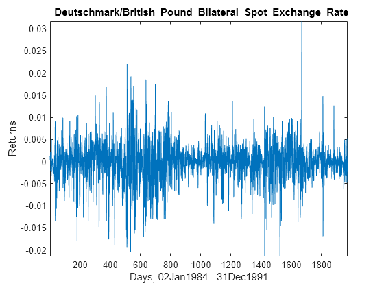
Convert the prices to returns, and plot the return series.

returns = price2ret(Data);

figure
plot(returns)
axis tight
ylabel('Returns')
xlabel('Days, 02Jan1984 - 31Dec1991')
title('{\bf Deutschmark/British Pound Bilateral Spot Exchange Rate}')

The returns series shows signs of heteroscedasticity.

Suppose that a GARCH(1,1) model is an appropriate model for the data. Fit a GARCH(1,1) model to the data including a constant.

Mdl = garch(1,1);
[EstMdl,EstParamCov] = estimate(Mdl,returns);

 
    GARCH(1,1) Conditional Variance Model (Gaussian Distribution):
 
                  Value       StandardError    TStatistic      PValue  
                __________    _____________    __________    __________

    Constant    1.0855e-06     3.5474e-07        3.0599       0.0022142
    GARCH{1}       0.80451       0.013132        61.264               0
    ARCH{1}         0.1545        0.01162        13.296      2.4419e-40

g1 = EstMdl.GARCH{1};
a1 = EstMdl.ARCH{1};

g1 is the estimated GARCH effect, and a1 is the estimated ARCH effect.

The following might represent relationships between the GARCH and ARCH coefficients:

• $${\gamma }_1{\alpha }_1=1$$

• $${\gamma }_1+{\alpha }_1=1$$

where $${\gamma }_1$$ is the GARCH effect and $${\alpha }_1$$ is the ARCH effect. Specify these relationships as the restriction function $$r(\theta )=0$$, evaluated at the unrestricted model parameter estimates. This specification defines a nested, restricted model.

r = [g1*a1; g1+a1] - 1;

Specify the Jacobian of the restriction function vector.

R = [0, a1, g1;0, 1, 1];

Conduct a Wald test to assess whether there is sufficient evidence to reject the restricted model.

[h,pValue,stat,cValue] = waldtest(r,R,EstParamCov)

h = logical
   1

pValue = 
0

stat = 
1.4450e+04

cValue = 
5.9915

h = 1 indicates that there is sufficient evidence to reject the restricted model in favor of the unrestricted model. pValue = 0 indicates that the evidence for rejecting the restricted model is strong.

Input Arguments

r — Restriction functions

scalar | vector | cell vector of scalars or vectors

Restriction functions corresponding to restricted models, specified as a scalar, vector, or cell vector of scalars or vectors.

• If r is a q-vector or a singleton cell array containing a q-vector, then the software conducts one Wald test. q must be less than the number of unrestricted model parameters.

• If r is a cell vector of length k > 1, and cell j contains a q_j-vector, j = 1,...,k, then the software conducts k independent Wald tests. Each q_j must be less than the number of unrestricted model parameters.

Data Types: double | cell

R — Restriction function Jacobians

row vector | matrix | cell vector of row vectors or matrices

Restriction function Jacobians, specified as a row vector, matrix, or cell vector of row vectors or matrices.

• Suppose r₁,...,r_q are the q restriction functions, and the unrestricted model parameters are θ₁,...,θ_p. Then, the restriction function Jacobian is

  $$R=\left(\begin{array}{ccc}\frac{\partial r_1}{\partial {\theta }_1}& \dots & \frac{\partial r_1}{\partial {\theta }_p}\\ ⋮& \ddots & ⋮\\ \frac{\partial r_q}{\partial {\theta }_1}& \cdots & \frac{\partial r_q}{\partial {\theta }_p}\end{array}\right).$$

• If R is a q-by-p matrix or a singleton cell array containing a q-by-p matrix, then the software conducts one Wald test. q must be less than p, which is the number of unrestricted model parameters.

• If R is a cell vector of length k > 1, and cell j contains a q_j-by-p_j matrix, j = 1,...,k, then the software conducts k independent Wald tests. Each q_j must be less than p_j, which is the number of unrestricted parameters in model j.

Data Types: double | cell

EstCov — Unrestricted model parameter covariance estimate

matrix | cell vector of matrices

Unrestricted model parameter covariance estimates, specified as a matrix or cell vector of matrices.

• If EstCov is a p-by-p matrix or a singleton cell array containing a p-by-p matrix, then the software conducts one Wald test. p is the number of unrestricted model parameters.

• If EstCov is a cell vector of length k > 1, and cell j contains a p_j-by-p_j matrix, j = 1,...,k, then the software conducts k independent Wald tests. Each p_j is the number of unrestricted parameters in model j.

Data Types: double | cell

alpha — Nominal significance levels

0.05 (default) | scalar | vector

Nominal significance levels for the hypothesis tests, specified as a scalar or vector.

Each element of alpha must be greater than 0 and less than 1.

When conducting k > 1 tests,

• If alpha is a scalar, then the software expands it to a k-by-1 vector.

• If alpha is a vector, then it must have length k.

Data Types: double

Output Arguments

h — Test rejection decisions

logical | vector of logicals

Test rejection decisions, returned as a logical value or vector of logical values with a length equal to the number of tests that the software conducts.

• h = 1 indicates rejection of the null, restricted model in favor of the alternative, unrestricted model.

• h = 0 indicates failure to reject the null, restricted model.

pValue — Test statistic p-values

scalar | vector

Test statistic p-values, returned as a scalar or vector with a length equal to the number of tests that the software conducts.

stat — Test statistics

scalar | vector

Test statistics, returned as a scalar or vector with a length equal to the number of tests that the software conducts.

cValue — Critical values

scalar | vector

Critical values determined by alpha, returned as a scalar or vector with a length equal to the number of tests that the software conducts.

More About

Wald Test

The Wald test compares specifications of nested models by assessing the significance of q parameter restrictions to an extended model with p unrestricted parameters.

The test statistic is

$$W=r^{\prime }{\left(R{\Sigma }_{\widehat{\theta }}{R}^{\prime }\right)}^{-1}r,$$

where

• r is the restriction function that specifies restrictions of the form r(θ) = 0 on parameters θ in the unrestricted model, evaluated at the unrestricted model parameter estimates. In other words, r maps the p-dimensional parameter space to the q-dimensional restriction space.

  In practice, r is a q-by-1 vector, where q < p.

  Usually, $$r=\widehat{\theta }-{\theta }_0$$, where $$\widehat{\theta }$$ is the unrestricted model parameter estimates for the restricted parameters and θ₀ holds the values of the restricted model parameters under the null hypothesis.

• R is the restriction function Jacobian evaluated at the unrestricted model parameter estimates.

• $${\widehat{\Sigma }}_{\widehat{\theta }}$$ is the unrestricted model parameter covariance estimator evaluated at the unrestricted model parameter estimates.

• W has an asymptotic chi-square distribution with q degrees of freedom.

When W exceeds a critical value in its asymptotic distribution, the test rejects the null, restricted hypothesis in favor of the alternative, unrestricted hypothesis. The nominal significance level (α) determines the critical value.

Note

Wald tests depend on the algebraic form of the restrictions. For example, you can express the restriction ab = 1 as a – 1/b = 0, or b – 1/a = 0, or ab – 1 = 0. Each formulation leads to different test statistics.

Tips

• Estimate unrestricted univariate linear time series models, such as arima or garch, or time series regression models (regARIMA) using estimate. Estimate unrestricted multivariate linear time series models, such as varm or vecm, using estimate.

  estimate returns parameter estimates and their covariance estimates, which you can process and use as inputs to waldtest.

• If you cannot easily compute restricted parameter estimates, then use waldtest. By comparison:

  • lratiotest requires both restricted and unrestricted parameter estimates.

  • lmtest requires restricted parameter estimates.

Algorithms

• waldtest performs multiple, independent tests when the restriction function vector, its Jacobian, and the unrestricted model parameter covariance matrix (r, R, and EstCov, respectively) are equal-length cell vectors.

  • If EstCov is the same for all tests, but r varies, then waldtest “tests down” against multiple restricted models.

  • If EstCov varies among tests, but r does not, then waldtest “tests up” against multiple unrestricted models.

  • Otherwise, waldtest compares model specifications pair-wise.

• alpha is nominal in that it specifies a rejection probability in the asymptotic distribution. The actual rejection probability is generally greater than the nominal significance.

• The Wald test rejection error is generally greater than the likelihood ratio and Lagrange multiplier test rejection errors.

References

[1] Davidson, R. and J. G. MacKinnon. Econometric Theory and Methods. Oxford, UK: Oxford University Press, 2004.

[2] Godfrey, L. G. Misspecification Tests in Econometrics. Cambridge, UK: Cambridge University Press, 1997.

[3] Greene, W. H. Econometric Analysis. 6th ed. Upper Saddle River, NJ: Pearson Prentice Hall, 2008.

[4] Hamilton, J. D. Time Series Analysis. Princeton, NJ: Princeton University Press, 1994.

Version History

Introduced in R2009a