Simulate Trend-Stationary and Difference-Stationary Processes
This example shows how to simulate trend-stationary and difference-stationary processes. The simulation results illustrate the distinction between these two nonstationary process models.
Generate Observations from Trend-Stationary Process
Specify the trend-stationary process
where the innovation process is Gaussian with variance 8. After specifying the model, simulate 50 sample paths of length 200. Use 100 burn-in simulations.
t = [1:200]';
trend = 0.5*t;

MdlTS = arima('Constant',0,'MA',{1.4,0.8},'Variance',8);
rng('default')
u = simulate(MdlTS,300,'NumPaths',50);

Yt = repmat(trend,1,50) + u(101:300,:);


figure
plot(Yt,'Color',[.85,.85,.85])
hold on
h1 = plot(t,trend,'r','LineWidth',5);
xlim([0,200])
title('Trend-Stationary Process')
h2 = plot(mean(Yt,2),'k--','LineWidth',2);
legend([h1,h2],'Trend','Simulation Mean',...
       'Location','NorthWest')
hold off

The sample paths fluctuate around the theoretical trend line with constant variance. The simulation mean is close to the true trend line.
Generate Observations from Difference-Stationary Process
Specify the difference-stationary model
where the innovation distribution is Gaussian with variance 8. After specifying the model, simulate 50 sample paths of length 200. No burn-in is needed because all sample paths should begin at zero. This is the simulate default starting point for nonstationary processes with no presample data.
MdlDS = arima('Constant',0.5,'D',1,'MA',{1.4,0.8},...
    'Variance',8);
Yd = simulate(MdlDS,200,'NumPaths',50);
figure
plot(Yd,'Color',[.85,.85,.85])
hold on
h1=plot(t,trend,'r','LineWidth',5);
xlim([0,200])
title('Difference-Stationary Process')
h2=plot(mean(Yd,2),'k--','LineWidth',2);
legend([h1,h2],'Trend','Simulation Mean',...
       'Location','NorthWest')
hold off
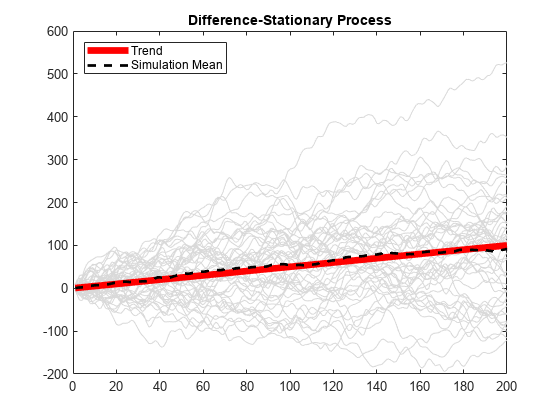
The simulation average is close to the trend line with slope 0.5. The variance of the sample paths grows over time.
Difference Sample Paths
A difference-stationary process is stationary when differenced appropriately. Take the first differences of the sample paths from the difference-stationary process, and plot the differenced series. One observation is lost as a result of the differencing.
diffY = diff(Yd,1,1);

figure
plot(2:200,diffY,'Color',[.85,.85,.85])
xlim([0,200])
title('Differenced Series')
hold on
h = plot(2:200,mean(diffY,2),'k--','LineWidth',2);
legend(h,'Simulation Mean','Location','NorthWest')
hold off
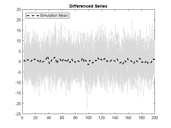
The differenced series appears stationary, with the simulation mean fluctuating around zero.