Fit Bayesian Stochastic Volatility Model to S&P 500 Volatility

This example fits a Bayesian stochastic volatility model to daily S&P 500 closing returns, and then it forecasts the volatility into a two-week horizon.

Load and Preprocess Data

Load the data set Data_GlobalIdx1.mat, which contains daily closing prices of selected global equity indices spanning trading dates 1993-04-27 through 2003-07-14. Extract the S&P 500 closing prices, which is the last column of the matrix Data.

load Data_GlobalIdx1
sp500 = Data(:,end);
T = numel(sp500);
dts = datetime(dates,ConvertFrom="datenum");

Plot the series.

figure
plot(dts,sp500)
title("S&P 500 Closing Prices")
ylabel("Closing Price (USD)")

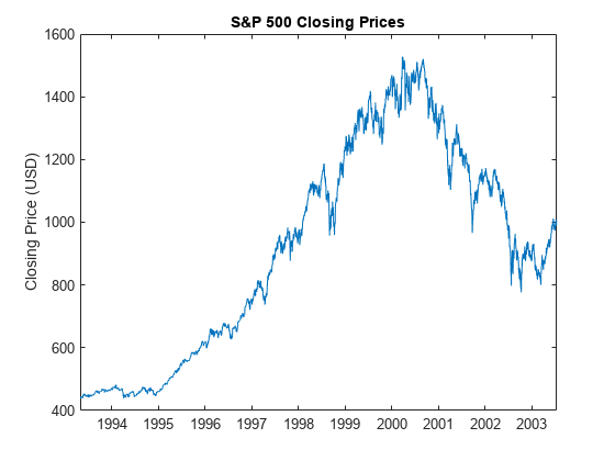
The series appears to be a random walk process; such processes are difficult to predict in levels. However, asset price series can exhibit volatility clustering, where price changes tend to be followed by price changes of similar magnitudes. The squared returns of an asset price series can exhibit predictable patterns, an exploitable characteristic for volatility forecasting.

Convert the price series to returns. Plot the returns.

retsp500 = price2ret(sp500);
retdts = dts(2:end);

figure
plot(retdts,100*retsp500)
title("S&P 500 Daily Returns")
ylabel("Return (%)")

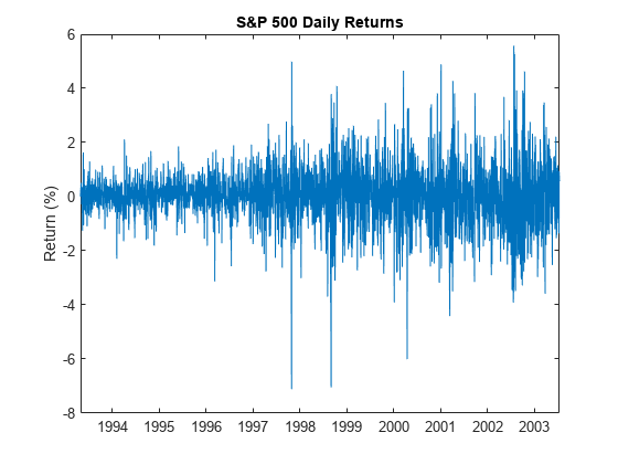
The plot indicates that price changes of similar magnitudes tend to follow each other.

Determine further whether the returns have serial correlation and volatility cluster further by plotting the autocorrelation function (ACF) of the returns series and its square.

figure
autocorr(retsp500)

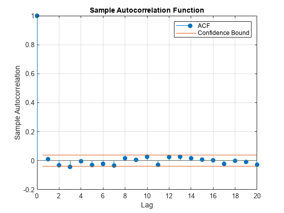
figure
autocorr(retsp500.^2)

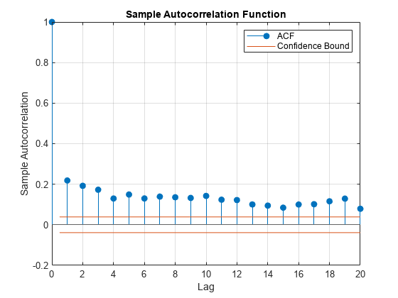
The correlogram of the returns indicates that no significant serial correlation exists in the series. However, the correlogram of the squared returns shows persistent serial correlation, which indicates that volatility clustering exists in the returns.

Create Bayesian State-Space Model

Econometric Toolbox™ has a suite of Conditional Variance Models objects (for example, garch object represents a GARCH model) that model volatility clustering when the observation innovations process is an iid Gaussian or Student's $\mathit{t}$ random series. However, a limitation of the GARCH model and its extensions is, given returns up to time $\mathit{t}-1$, the conditional variance of the return at time $\mathit{t}$ is not stochastic.

The stochastic volatility model, which also models volatility clustering is asset returns series, can capture richer characteristics in the series because the conditional variance at time $\mathit{t}$ is random, even given all past asset prices. Unlike the GARCH model, the likelihood of a stochastic volatility model is analytically intractable, which makes estimation difficult.

The stochastic volatility model for observed asset returns ${\mathit{y}}_{\mathit{t}}$ has the following nonlinear state-space form

$$\begin{array}{l}{x}_{t+\Delta t}=\alpha +\beta x_t+\sigma u_t\\ y_t=exp\left(\frac{1}{2}{x}_t\right)\sqrt{\Delta t}{\epsilon }_t,\end{array}$$

where:

• $\Delta \mathit{t}=\frac{1}{365}$ for daily returns.

• ${\mathit{x}}_{\mathit{t}}$ is a latent AR(1) process representing the conditional volatility series.

• ${\mathit{u}}_{\mathit{t}}$ are ${\epsilon }_{\mathit{t}}$ are mutually independent and individually iid random standard Gaussian noise series.

Econometrics Toolbox state-space model functionalities support linear state-space models. To linearize the model, square and then apply the log transform to both sides of the observation equation.

$$\log {\mathit{y}}_{\mathit{t}}^2=\log \sqrt{\Delta \mathit{t}}+{\mathit{x}}_{\mathit{t}}+\log {\epsilon }_{\mathit{t}}^2.$$

The random variable ${\nu }_{\mathit{t}}=\log {\epsilon }_{\mathit{t}}^2$ has a $\log {\chi }_1^2$ distribution, which is well approximated by a properly configured 7-regime Gaussian mixture model. Although the resulting model is linear with respect to the parameters, the loglikelihood is intractable. The bssm framework supports a Bayesian view of the model, which accommodates intractable loglikelihoods by implementing Markov chain Monte Carlo (MCMC) methods, such as Metropolis-within-Gibbs sampling.

bssm requires the following inputs:

• A function specifying the state-space model structure. The function accepts an input vector theta and returns coefficient matrices, initial state moments, and a flag indicating whether the state is stationary.

• A function specifying the log prior distribution of the state-space model parameters theta, from which to compose the posterior distribution. The function accepts theta and returns the scalar log prior evaluated at theta.

The state-space model has two states $\left[\begin{array}{cc}{\mathit{x}}_{\mathit{t}}& 1\end{array}\right]\prime$, a stationary state ${\mathit{x}}_{\mathit{t}}$ and a state that always takes the value 1 to identify $\alpha$, and three parameters, $\alpha$, $\beta$, and $\sigma$. The coefficient matrices are:

• $$\mathit{A}=\left[\begin{array}{cc}\beta & \alpha \\ 0& 1\end{array}\right].$$

• $$\mathit{B}=\left[\begin{array}{c}\sigma \\ 0\end{array}\right].$$

• $$\mathit{C}=\left[\begin{array}{cc}1& -\log \left(365\right)\end{array}\right].$$

• $$\mathit{D}=1.$$

The local function paramMap specifies this model structure.

Assume a flat prior, that is, the log prior is 0 over the support of the parameters and -Inf everywhere else. The local function flatPriorBSSM specifies the prior.

Create a Bayesian state-space model that specifies the model structure and prior distribution. Approximate the $\log {\chi }_1^2$ distributed observation innovations by specifying that their distribution is a 7-regime finite Gaussian mixture with the following parameter settings:

• Regime weight vector is [0.0089 0.0541 0.1338 0.2761 0.2923 0.1494 0.0854]

• Regime mean vector is [-9.3202 -5.3145 -3.4147 -1.7097 -0.4531 0.3975 1.1925]

• Regime variance vector is [3.2793 2.4574 1.8874 1.3121 0.8843 0.5898 0.4995].^2

weight = [0.0089 0.0541 0.1338 0.2761 0.2923 0.1494 0.0854];
mu = [-9.3202 -5.3145 -3.4147 -1.7097 -0.4531 0.3975 1.1925];
sigma2 = [3.2793 2.4574 1.8874 1.3121 0.8843 0.5898 0.4995].^2;

ObsInnovDist = struct("Name","mixture","Weight",weight, ...
    "Mean",mu,"Variance",sigma2);
PriorMdl = bssm(@paramMap,@flatPriorBSSM,ObservationDistribution=ObsInnovDist);

Estimate Posterior Distribution

Several consecutive days resulted in no change in price, which correspond to -Inf changes on the log-returns scale. Such observations cause computational problems during MCMC sampling.

To avoid -Inf log returns, center the returns before applying the squared log transformation.

y = 2*log(abs(retsp500-mean(retsp500)));

Estimate the posterior distribution of the parameters. estimate uses the Metropolis-within-Gibbs sampler to generate a sample from the posterior. To generate a good quality sample, you must tune the sampler carefully. Specify the following settings:

• Specify the univariate treatment of mutlivariate states.

• Use the outer product of gradients to approximate the Hessian.

• Specify a burn-in period of 10000 draws.

• Specify a sample thinning factor of 25.

Return the posterior distribution, the Bayesian parameter estimates and their estimated covariance matrix, and draws of all parameters and the final states. The sampler, with these settings, takes some time to complete.

theta0 = [0.2 0 0.5];
burnin = 10000;
thin = 25;

rng(1)
[PosteriorMdl,estParams,EstParamCov,PostSumry] = estimate(PriorMdl,y, ...
    theta0,Univariate=true,Hessian="opg",BurnIn=burnin,Thin=thin);

Local minimum possible.

fminunc stopped because the size of the current step is less than
the value of the step size tolerance.

         Optimization and Tuning        
      | Params0  Optimized  ProposalStd 
----------------------------------------
 c(1) |  0.2000    0.9962      0.0019   
 c(2) |   0       -0.0189      0.0097   
 c(3) |  0.5000    0.0856      0.0140   
 
             Posterior Distributions            
      |   Mean     Std   Quantile05  Quantile95 
------------------------------------------------
 c(1) |  0.9892  0.0038     0.9821      0.9945  
 c(2) | -0.0391  0.0141    -0.0649     -0.0194  
 c(3) |  0.1345  0.0190     0.1060      0.1679  
 x(1) | -3.4679  0.4194    -4.1322     -2.7680  
 x(2) |   1       0          1           1      
Proposal acceptance rate = 43.82%

Assess Quality of Posterior Sample

Determine the quality of the posterior sample by plotting trace plots of the parameter draws.

figure
plot(PosteriorMdl.ParamDistribution(1,:))
title("Trace Plot: \beta")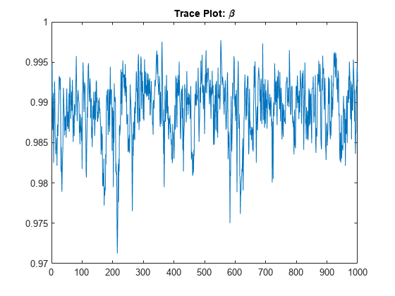

figure
plot(PosteriorMdl.ParamDistribution(2,:))
title("Trace Plot: \alpha")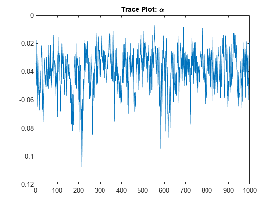

figure
plot(PosteriorMdl.ParamDistribution(3,:))
title("Trace Plot: \sigma")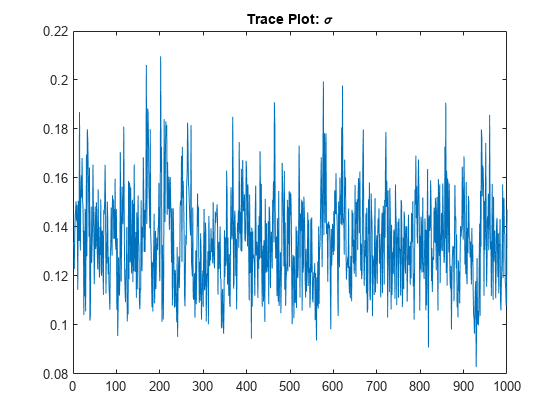

The posterior samples show good mixing with some minor serial correlation.

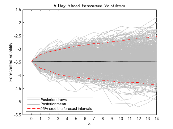
Forecast Volatility

Draw a large sample from the posterior distribution of forecasted volatility ${\stackrel{\sim }{\mathit{x}}}_{\mathit{t},\mathit{j}}$ into a 14 day horizon by using the equation

$${\underset{}{\overset{\sim }{x}}}_{t,j}={\underset{}{\overset{\sim }{\alpha }}}_j+{\underset{}{\overset{\sim }{\beta }}}_j{\underset{}{\overset{\sim }{x}}}_{t-1,j}+{\underset{}{\overset{\sim }{\sigma }}}_j{u}_{t,j}$$,

where:

• ${\stackrel{\sim }{\alpha }}_{\mathit{j}}$, ${\stackrel{\sim }{\beta }}_{\mathit{j}}$, and ${\stackrel{\sim }{\sigma }}_{\mathit{j}}$ are individual draws from the posterior distribution of the corresponding parameter.

• ${\mathit{u}}_{\mathit{t},\mathit{j}}\sim \mathit{N}\left(0,1\right)$.

fh = 14;
bigN = 1000;
XF = zeros(fh + 1,bigN);
XF(1,:) = PostSumry.Mean(4)*ones(1,bigN);  
betatilde = PosteriorMdl.ParamDistribution(1,(end-(bigN-1)):end);
alphatilde = PosteriorMdl.ParamDistribution(2,(end-(bigN-1)):end);
sigmatilde = PosteriorMdl.ParamDistribution(3,(end-(bigN-1)):end);
for j = 2:(fh+1)
    XF(j,:) = alphatilde + betatilde.*XF(j-1,:) + sigmatilde.*randn(1,bigN);
end

Summarize the posterior distribution of the forecasts by computing the mean of each step into the horizon and the 95% percentile-based credible forecast intervals.

xfmean = mean(XF,2);
XFCI = quantile(XF,[0.025 0.975],2);
array2table([xfmean XFCI],VariableNames=["PostMean" "CILower" "CIUpper"])

ans=15×3 table
    PostMean    CILower    CIUpper
    ________    _______    _______

    -3.4679     -3.4679    -3.4679
    -3.4743     -3.7319    -3.2137
    -3.4721     -3.8313    -3.0995
    -3.4766     -3.9682    -3.0329
    -3.4788     -4.0266    -2.9581
    -3.4765     -4.0736    -2.8724
     -3.478     -4.0979    -2.8503
    -3.4758     -4.1471     -2.786
    -3.4778     -4.1913    -2.7804
    -3.4854     -4.2174    -2.7212
    -3.4797     -4.2807    -2.6942
    -3.4824     -4.2763    -2.6341
    -3.4829     -4.2683    -2.5818
     -3.482     -4.3311    -2.5722
     -3.485     -4.3667    -2.5182

figure
h1 = plot(XF,Color=[0.75 0.75 0.75]);
hold on
h2 = plot(xfmean,"k");
h3 = plot(XFCI,"r--");
title("$h$-Day-Ahead Forecasted Volatilities",Interpreter="latex")
xticks(1:(fh+1))
xticklabels(0:fh)
xlabel("$h$",Interpreter="latex")
ylabel("Forecasted Volatility")
legend([h1(1) h2 h3(1)], ...
    ["Posterior draws" "Posterior mean" "95% credible forecast intervals"], ...
    Location="southwest")

Local Functions

This example uses the following functions. paramMap is the parameter-to-matrix mapping function and priorDistribution is the log prior distribution of the parameters.

function [A,B,C,D,Mean0,Cov0,StateType] = paramMap(theta)
    A = [theta(1) theta(2); 0 1];
    B = [theta(3); 0];
    C = [1 -log(365)];
    D = 1;
    Mean0 = [];         % MATLAB uses default initial state mean
    Cov0 = [];          % MATLAB uses initial state covariances
    StateType = [0; 1]; % x is stationary and the constant 1 state for alpha
end

function logprior = flatPriorBSSM(theta)
% flatPriorBSSM computes the log of the flat prior density for the three
% variables in theta. Log probabilities for parameters outside the
% parameter space are -Inf.
    paramcon = zeros(numel(theta),1);
    % theta(1) is the lag 1 term in a stationary AR(1) model. The
    % value needs to be within the unit circle.
    paramcon(1) = abs(theta(1)) >= 1 - eps;

    % alpha must be finite
    paramcon(2) = ~isfinite(theta(2)); 

    % Standard deviation of the state disturbance theta(3) must be positive.
    paramcon(3) = theta(3) <= eps;

    if sum(paramcon) > 0
        logprior = -Inf;
    else
        logprior = 0;   % Prior density is proportional to 1 for all values
                        % in the parameter space.
    end
end