Adaptive Noise Cancellation Using RLS Adaptive Filtering

This example shows how to use an RLS filter to extract useful information from a noisy signal. The information bearing signal is a sine wave that is corrupted by additive white Gaussian noise.

The adaptive noise cancellation system assumes the use of two microphones. A primary microphone picks up the noisy input signal, while a secondary microphone receives noise that is uncorrelated to the information bearing signal but is correlated to the noise picked up by the primary microphone.

Note: This example is equivalent to the Simulink® model rlsdemo provided.

The model illustrates the ability of the adaptive RLS filter to extract useful information from a noisy signal.

The information bearing signal is a sine wave of 0.055 cycles/sample. Create the information bearing signal and plot it.

signal = sin(2*pi*0.055*(0:1000-1)');
signalSource = dsp.SignalSource(signal,SamplesPerFrame=100,...
    SignalEndAction="Cyclic repetition");
scope = timescope(YLimits=[-2 2],Title="Information bearing signal")

scope = 
  timescope handle with properties:

               SampleRate: 1
           TimeSpanSource: 'auto'
    TimeSpanOverrunAction: 'scroll'
                 PlotType: 'line'
              AxesScaling: 'manual'

  Show all properties

scope(signal(1:200));

The noise picked up by the secondary microphone is the input to the RLS adaptive filter. The noise that corrupts the sine wave is a lowpass filtered version of (correlated to) this noise. The sum of the filtered noise and the information bearing signal is the desired signal for the adaptive filter. Create the noise signal and plot it.

nvar  = 1.0;                  % Noise variance
noise = randn(1000,1)*nvar;   % White noise
noiseSource = dsp.SignalSource(noise,SamplesPerFrame=100,...
    SignalEndAction="Cyclic repetition");
scope = timescope(YLimits=[-4 4], Title="Noise picked up by the secondary microphone");
scope(noise);

The noise corrupting the information bearing signal is a filtered version of the noise signal you created in the previous step. Initialize the filter that operates on the noise signal.

lp = dsp.FIRFilter('Numerator',fir1(31,0.5));% Low pass FIR filter

Set the parameters of the RLS filter and initialize the filter.

M      = 32;                 % Filter order
delta  = 0.1;                % Initial input covariance estimate
P0     = (1/delta)*eye(M,M); % Initial setting for the P matrix
rlsfilt = dsp.RLSFilter(M,InitialInverseCovariance=P0);

Run the RLS adaptive filter for 1000 iterations. As the adaptive filter converges, the filtered noise should be completely subtracted from signal + noise. The error e should contain only the original signal.

scope = timescope(TimeSpan=1000,YLimits=[-2,2], ...
	              TimeSpanOverrunAction="scroll");
for k = 1:10
    n = noiseSource(); % Noise
    s = signalSource();
    d = lp(n) + s;
    [y,e]  = rlsfilt(n,d);
    scope([s,e]);
end
release(scope);

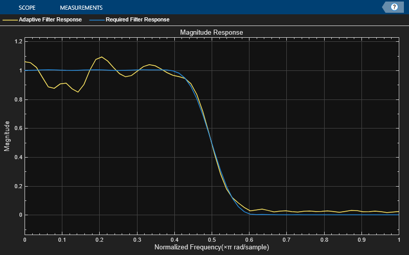
The plot shows the convergence of the adaptive filter response to the response of the FIR filter.

visualizer = dsp.DynamicFilterVisualizer(64,NormalizedFrequency=true,...
    MagnitudeDisplay="Magnitude", ...
    FilterNames=["Adaptive Filter Response","Required Filter Response"]);
visualizer(rlsfilt.Coefficients,1,lp.Numerator,1);

References

[1] S.Haykin, "Adaptive Filter Theory", 3rd Edition, Prentice Hall, N.J., 1996.