Noise Cancellation Using Sign-Data LMS Algorithm
When the amount of computation required to derive an adaptive filter drives your development process, the sign-data variant of the LMS (SDLMS) algorithm might be a very good choice, as demonstrated in this example.
In the standard and normalized variations of the LMS adaptive filter, coefficients for the adapting filter arise from the mean square error between the desired signal and the output signal from the unknown system. The sign-data algorithm changes the mean square error calculation by using the sign of the input data to change the filter coefficients.
When the error is positive, the new coefficients are the previous coefficients plus the error multiplied by the step size µ. If the error is negative, the new coefficients are again the previous coefficients minus the error multiplied by µ — note the sign change.
When the input is zero, the new coefficients are the same as the previous set.
In vector form, the sign-data LMS algorithm is:
where
with vector containing the weights applied to the filter coefficients and vector containing the input data. The vector is the error between the desired signal and the filtered signal. The objective of the SDLMS algorithm is to minimize this error. Step size is represented by .
With a smaller , the correction to the filter weights gets smaller for each sample, and the SDLMS error falls more slowly. A larger changes the weights more for each step, so the error falls more rapidly, but the resulting error does not approach the ideal solution as closely. To ensure a good convergence rate and stability, select within the following practical bounds.
where is the number of samples in the signal. Also, define as a power of two for efficient computing.
Note: How you set the initial conditions of the sign-data algorithm profoundly influences the effectiveness of the adaptation process. Because the algorithm essentially quantizes the input signal, the algorithm can become unstable easily.
A series of large input values, coupled with the quantization process might result in the error growing beyond all bounds. Restrain the tendency of the sign-data algorithm to get out of control by choosing a small step size and setting the initial conditions for the algorithm to nonzero positive and negative values.
In this noise cancellation example, set the Method property of dsp.LMSFilter to 'Sign-Data LMS'. This example requires two input data sets:
Data containing a signal corrupted by noise. In the block diagram under Noise or Interference Cancellation –– Using an Adaptive Filter to Remove Noise from an Unknown System, this is the desired signal . The noise cancellation process removes the noise from the signal.
Data containing random noise. In the block diagram under Noise or Interference Cancellation –– Using an Adaptive Filter to Remove Noise from an Unknown System, this is . The signal is correlated with the noise that corrupts the signal data. Without the correlation between the noise data, the adapting algorithm cannot remove the noise from the signal.
For the signal, use a sine wave. Note that signal is a column vector of 1000 elements.
signal = sin(2*pi*0.055*(0:1000-1)');
Now, add correlated white noise to signal. To ensure that the noise is correlated, pass the noise through a lowpass FIR filter and then add the filtered noise to the signal.
noise = randn(1000,1);
filt = dsp.FIRFilter;
filt.Numerator = fir1(11,0.4);
fnoise = filt(noise);
d = signal + fnoise;
fnoise is the correlated noise and d is now the desired input to the sign-data algorithm.
To prepare the dsp.LMSFilter object for processing, set the initial conditions of the filter weights and mu (StepSize). As noted earlier in this section, the values you set for coeffs and mu determine whether the adaptive filter can remove the noise from the signal path.
In System Identification of FIR Filter Using LMS Algorithm, you constructed a default filter that sets the filter coefficients to zeros. In most cases that approach does not work for the sign-data algorithm. The closer you set your initial filter coefficients to the expected values, the more likely it is that the algorithm remains well behaved and converges to a filter solution that removes the noise effectively.
For this example, start with the coefficients used in the noise filter (filt.Numerator), and modify them slightly so the algorithm has to adapt.
coeffs = (filt.Numerator).'-0.01; % Set the filter initial conditions.
mu = 0.05; % Set the step size for algorithm updating.
With the required input arguments for dsp.LMSFilter prepared, construct the LMS filter object, run the adaptation, and view the results.
lms = dsp.LMSFilter(12,'Method','Sign-Data LMS',...
   'StepSize',mu,'InitialConditions',coeffs);
[~,e] = lms(noise,d);
L = 200;
plot(0:L-1,signal(1:L),0:L-1,e(1:L));
title('Noise Cancellation by the Sign-Data Algorithm');
legend('Actual signal','Result of noise cancellation',...
       'Location','NorthEast');
xlabel('Time index')
ylabel('Signal values')
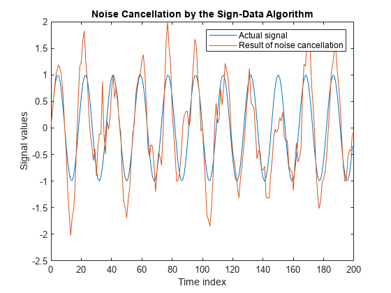
When dsp.LMSFilter runs, it uses far fewer multiplication operations than either of the standard LMS algorithms. Also, performing the sign-data adaptation requires only multiplication by bit shifting when the step size is a power of two.
Although the performance of the sign-data algorithm as shown in this plot is quite good, the sign-data algorithm is much less stable than the standard LMS variations. In this noise cancellation example, the processed signal is a very good match to the input signal, but the algorithm could very easily grow without bound rather than achieve good performance.
Changing the weight initial conditions (InitialConditions) and mu (StepSize), or even the lowpass filter you used to create the correlated noise, can cause noise cancellation to fail.
See Also
Objects
Topics
- Noise Cancellation Using Sign-Error LMS Algorithm
- Noise Cancellation Using Sign-Sign LMS Algorithm
- System Identification of FIR Filter Using LMS Algorithm
References
[1] Hayes, Monson H., Statistical Digital Signal Processing and Modeling. Hoboken, NJ: John Wiley & Sons, 1996, pp.493–552.
[2] Haykin, Simon, Adaptive Filter Theory. Upper Saddle River, NJ: Prentice-Hall, Inc., 1996.