Weight Tying Using Nested Layer

This example shows how to implement weight tying using a nested layer.

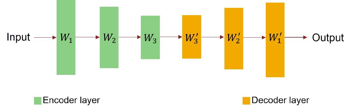
When two separate layers in a neural network have similar properties with respect to the input data, for example, when they learn similar features, the layers can share the same weights. This is typically referred to as weight tying and is commonly used in language models [1] and autoencoders [2]. The network in this example is an autoencoder, as illustrated in the figure below, and weight tying is implemented using a nested layer. For information on nested layer, see Define Nested Deep Learning Layer Using Network Composition.

Load Data

The data set contains synthetic images of handwritten digits.

Load the training and test data from the MAT files DigitsDataTrain.mat and DigitsDataTest.mat, respectively. The training and test data sets each contain 5000 images.

load DigitsDataTrain.mat
load DigitsDataTest.mat

View the size of each image in the training data

inputSize = size(XTrain, [1 2 3])

inputSize = 1×3

    28    28     1

Partition the test data into a validation set containing 60% of the test data and a test set containing the remaining 40% of the data. To partition the data, use the trainingPartitions function, attached to this example as a supporting file. To access this file, open the example as a live script.

[idxValidation,idxTest] = trainingPartitions(size(XTest,4),[0.6,0.4]);
XValidation = XTest(:,:,:,idxValidation);
XTest = XTest(:,:,:,idxTest);

Define Network Architecture

Autoencoders consists of two separate networks, the encoder network that downsamples the input image into a latent representation, and the decoder network that reconstructs the image from the latent representation.

Define Encoder Network

Define the encoder network as a feed forward neural network as illustrated in the network architecture diagram below. In this diagram, W represents weights of the fully connected layers.

Set the output sizes of the fully connected layers to 784, 392, and 196, respectively.

encoderLayers = [
    fullyConnectedLayer(784)
    reluLayer
    fullyConnectedLayer(392)
    reluLayer
    fullyConnectedLayer(196)
    reluLayer];

Define Decoder Network

Define the decoder network using a similar architecture as the encoder network and tying the weights of the fully connected layers in the decoder network to the weights of the fully connected layers in the encoder network as illustrated in the diagram below. In this diagram, W' represents transposed weight W.

To tie the layer weights, create a custom layer that represents the full network (both the encoder and the decoder), defines the shared learnable parameters and defines the forward pass of the network in terms of these shared learnable parameters.

The custom layer weightTyingAutoEncoderLayer, attached to this example as a supporting file, takes an input image, performs a forward pass of the encoder network and then the decoder network using the transposed shared weights, and outputs the reconstructed image. To access this file, open the example as a live script.

The layer has these learnable parameters:

A nested network representing the encoder network .
The input bias for the decoder.
The hidden bias for the decoder .
The output bias for the decoder.

The layer hard-codes the decoder to network using dlarray functions that use the shared weights and the biases specified as learnable parameters. Note that only the weights are shared, the biases are not shared. To modify the encoder and decoder network architectures, make changes to the encoder layer array and the custom layer code, respectively.

Create a dlnetwork object that contains the custom layer. The training data is already normalized, so set the Normalization option of the input layer to "none".

layers = [imageInputLayer(inputSize, Normalization="none")
    weightTyingAutoEncoderLayer(encoderLayers)];

net = dlnetwork(layers);

Specify Training Options

Specify the training options. Choosing among the options requires empirical analysis. To explore different training option configurations by running experiments, you can use the Experiment Manager app.

Train using the Adam optimizer.
Validate the network using the validation data. For autoencoder workflows, the input data and targets match.
Display the training progress in a plot and monitor the root mean squared error metric.
Disable the verbose output.

options = trainingOptions("adam",...
    ValidationData={XValidation, XValidation},...
    Plots="training-progress",...
    Metrics="rmse",...
    Verbose=false);

Train Network

Train the neural network using the trainnet function. For image reconstruction, use binary cross-entropy loss. By default, the trainnet function uses a GPU if one is available. Using a GPU requires a Parallel Computing Toolbox™ license and a supported GPU device. For information on supported devices, see GPU Computing Requirements (Parallel Computing Toolbox). Otherwise, the function uses the CPU. To specify the execution environment, use the ExecutionEnvironment training option.

net = trainnet(XTrain,XTrain,net,"binary-crossentropy",options);

Test Network

Make predictions with the trained weight-tying autoencoder using the minibatchpredict function.

YTest = minibatchpredict(net, XTest);

Calculate the root-mean-square-error between the reconstructed images and the test images using the rmse function.

err = rmse(XTest,YTest,"all")

err = single
    0.0757

Randomly select and visualize samples of the original test images and their reconstructed versions.

numSamples = 5;
idx = randperm(size(XTest, 4), numSamples);
layout = tiledlayout(numSamples,2);
for n = 1:numSamples
    nexttile
    imshow(XTest(:,:,:,idx(n)))
    title("Original")
    nexttile
    imshow(YTest(:,:,:,idx(n)))
    title("Reconstructed")
end

References

Ofir Press, and Lior Wolf. “Using the Output Embedding to Improve Language Models.” In Proceedings of the 15th Conference of the European Chapter of the Association for Computational Linguistics, Valencia, Spain, April 2017.
Hinton, G.E., and Salakhutdinov, R.R. "Reducing the dimensionality of data with neural networks." Science 313(5786), 504–507 (2006).