Train Generative Adversarial Network (GAN)
This example shows how to train a generative adversarial network to generate images.
A generative adversarial network (GAN) is a type of deep learning network that can generate data with similar characteristics as the input real data.
The trainnet function does not support training GANs, so you must implement a custom training loop. To train the GAN using a custom training loop, you can use dlarray and dlnetwork objects for automatic differentiation.
A GAN consists of two networks that train together:
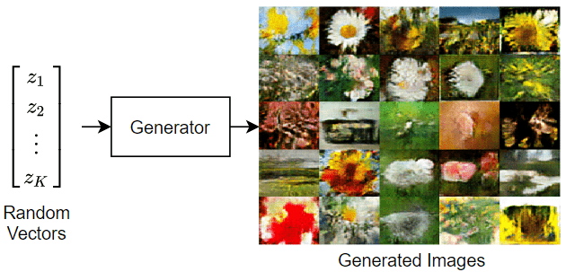
Generator — Given a vector of random values (latent inputs) as input, this network generates data with the same structure as the training data.
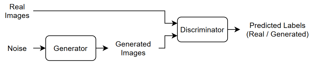
Discriminator — Given batches of data containing observations from both the training data, and generated data from the generator, this network attempts to classify the observations as
"real"or"generated".
This diagram illustrates the generator network of a GAN generating images from vectors of random inputs.
This diagram illustrates the structure of a GAN.
To train a GAN, train both networks simultaneously to maximize the performance of both:
Train the generator to generate data that "fools" the discriminator.
Train the discriminator to distinguish between real and generated data.
To optimize the performance of the generator, maximize the loss of the discriminator when given generated data. That is, the objective of the generator is to generate data that the discriminator classifies as "real".
To optimize the performance of the discriminator, minimize the loss of the discriminator when given batches of both real and generated data. That is, the objective of the discriminator is to not be "fooled" by the generator.
Ideally, these strategies result in a generator that generates convincingly realistic data and a discriminator that has learned strong feature representations that are characteristic of the training data.
This example trains a GAN to generate images using the Flowers data set [1], which contains images of flowers.
Load Training Data
Download and extract the Flowers data set [1].
url = "http://download.tensorflow.org/example_images/flower_photos.tgz";
downloadFolder = tempdir;
filename = fullfile(downloadFolder,"flower_dataset.tgz");

imageFolder = fullfile(downloadFolder,"flower_photos");
if ~datasetExists(imageFolder)
    disp("Downloading Flowers data set (218 MB)...")
    websave(filename,url);
    untar(filename,downloadFolder)
end
Create an image datastore containing the photos of the flowers.
imds = imageDatastore(imageFolder,IncludeSubfolders=true);
Augment the data to include random horizontal flipping and resize the images to have size 64-by-64.
augmenter = imageDataAugmenter(RandXReflection=true);
augimds = augmentedImageDatastore([64 64],imds,DataAugmentation=augmenter);
Define Generative Adversarial Network
A GAN consists of two networks that train together:
Generator — Given a vector of random values (latent inputs) as input, this network generates data with the same structure as the training data.
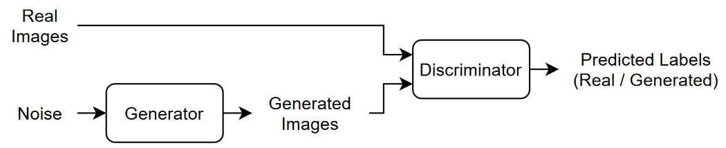
Discriminator — Given batches of data containing observations from both the training data, and generated data from the generator, this network attempts to classify the observations as
"real"or"generated".
This diagram illustrates the structure of a GAN.
Define Generator Network
Define the following network architecture, which generates images from random vectors.
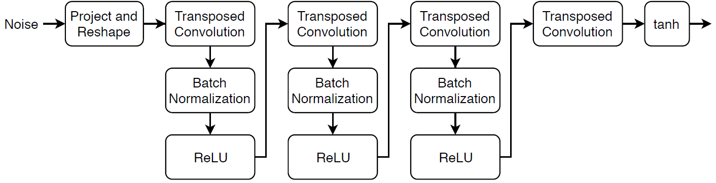
This network:
Converts the random vectors of size 100 to 4-by-4-by-512 arrays using a project and reshape operation.
Upscales the resulting arrays to 64-by-64-by-3 arrays using a series of transposed convolution layers with batch normalization and ReLU layers.
Define this network architecture as a layer graph and specify the following network properties.
For the transposed convolution layers, specify 5-by-5 filters with a decreasing number of filters for each layer, a stride of 2, and cropping of the output on each edge.
For the final transposed convolution layer, specify three 5-by-5 filters corresponding to the three RGB channels of the generated images, and the output size of the previous layer.
At the end of the network, include a tanh layer.
To project and reshape the noise input, use the custom layer projectAndReshapeLayer, attached to this example as a supporting file. To access this layer, open the example as a live script.
filterSize = 5;
numFilters = 64;
numLatentInputs = 100;

projectionSize = [4 4 512];

layersGenerator = [
    featureInputLayer(numLatentInputs)
    projectAndReshapeLayer(projectionSize)
    transposedConv2dLayer(filterSize,4*numFilters)
    batchNormalizationLayer
    reluLayer
    transposedConv2dLayer(filterSize,2*numFilters,Stride=2,Cropping="same")
    batchNormalizationLayer
    reluLayer
    transposedConv2dLayer(filterSize,numFilters,Stride=2,Cropping="same")
    batchNormalizationLayer
    reluLayer
    transposedConv2dLayer(filterSize,3,Stride=2,Cropping="same")
    tanhLayer];
To train the network with a custom training loop and enable automatic differentiation, convert the layer graph to a dlnetwork object.
netG = dlnetwork(layersGenerator);
Define Discriminator Network
Define the following network, which classifies real and generated 64-by-64 images.
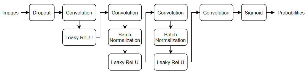
Create a network that takes 64-by-64-by-3 images and returns a scalar prediction score using a series of convolution layers with batch normalization and leaky ReLU layers. Add noise to the input images using dropout.
For the dropout layer, specify a dropout probability of 0.5.
For the convolution layers, specify 5-by-5 filters with an increasing number of filters for each layer. Also specify a stride of 2 and padding of the output.
For the leaky ReLU layers, specify a scale of 0.2.
To output the probabilities in the range [0,1], specify a convolutional layer with one 4-by-4 filter followed by a sigmoid layer.
dropoutProb = 0.5;
numFilters = 64;
scale = 0.2;

inputSize = [64 64 3];
filterSize = 5;

layersDiscriminator = [
    imageInputLayer(inputSize,Normalization="none")
    dropoutLayer(dropoutProb)
    convolution2dLayer(filterSize,numFilters,Stride=2,Padding="same")
    leakyReluLayer(scale)
    convolution2dLayer(filterSize,2*numFilters,Stride=2,Padding="same")
    batchNormalizationLayer
    leakyReluLayer(scale)
    convolution2dLayer(filterSize,4*numFilters,Stride=2,Padding="same")
    batchNormalizationLayer
    leakyReluLayer(scale)
    convolution2dLayer(filterSize,8*numFilters,Stride=2,Padding="same")
    batchNormalizationLayer
    leakyReluLayer(scale)
    convolution2dLayer(4,1)
    sigmoidLayer];
To train the network with a custom training loop and enable automatic differentiation, convert the layer graph to a dlnetwork object.
netD = dlnetwork(layersDiscriminator);
Define Model Loss Functions
Create the function modelLoss, listed in the Model Loss Function section of the example, which takes as input the generator and discriminator networks, a mini-batch of input data, an array of random values, and the flip factor, and returns the loss values, the gradients of the loss values with respect to the learnable parameters in the networks, the generator state, and the scores of the two networks.
Specify Training Options
Train with a mini-batch size of 128 for 500 epochs. For larger data sets, you might not need to train for as many epochs.
numEpochs = 500;
miniBatchSize = 128;
Specify the options for Adam optimization. For both networks, specify:
A learning rate of 0.0002
A gradient decay factor of 0.5
A squared gradient decay factor of 0.999
learnRate = 0.0002;
gradientDecayFactor = 0.5;
squaredGradientDecayFactor = 0.999;
If the discriminator learns to discriminate between real and generated images too quickly, then the generator can fail to train. To better balance the learning of the discriminator and the generator, add noise to the real data by randomly flipping the labels assigned to the real images.
Specify to flip the real labels with probability 0.35. Note that this does not impair the generator as all the generated images are still labeled correctly.
flipProb = 0.35;
Display the generated validation images every 100 iterations.
validationFrequency = 100;
Train Model
To train a GAN, train both networks simultaneously to maximize the performance of both:
Train the generator to generate data that "fools" the discriminator.
Train the discriminator to distinguish between real and generated data.
To optimize the performance of the generator, maximize the loss of the discriminator when given generated data. That is, the objective of the generator is to generate data that the discriminator classifies as "real".
To optimize the performance of the discriminator, minimize the loss of the discriminator when given batches of both real and generated data. That is, the objective of the discriminator is to not be "fooled" by the generator.
Ideally, these strategies result in a generator that generates convincingly realistic data and a discriminator that has learned strong feature representations that are characteristic of the training data.
Use minibatchqueue to process and manage the mini-batches of images. For each mini-batch:
Use the custom mini-batch preprocessing function
preprocessMiniBatch(defined at the end of this example) to rescale the images in the range[-1,1].Discard any partial mini-batches with fewer observations than the specified mini-batch size.
Format the image data with the format
"SSCB"(spatial, spatial, channel, batch). By default, theminibatchqueueobject converts the data todlarrayobjects with underlying typesingle.Train on a GPU if one is available. By default, the
minibatchqueueobject converts each output to agpuArrayif a GPU is available. Using a GPU requires Parallel Computing Toolbox™ and a supported GPU device. For information on supported devices, see GPU Computing Requirements (Parallel Computing Toolbox).
augimds.MiniBatchSize = miniBatchSize;

mbq = minibatchqueue(augimds, ...
    MiniBatchSize=miniBatchSize, ...
    PartialMiniBatch="discard", ...
    MiniBatchFcn=@preprocessMiniBatch, ...
    MiniBatchFormat="SSCB");
Train the model using a custom training loop. Loop over the training data and update the network parameters at each iteration. To monitor the training progress, display a batch of generated images using a held-out array of random values to input to the generator as well as a plot of the scores.
Initialize the parameters for Adam optimization.
trailingAvgG = [];
trailingAvgSqG = [];
trailingAvg = [];
trailingAvgSqD = [];
To monitor the training progress, display a batch of generated images using a held-out batch of fixed random vectors fed into the generator and plot the network scores.
Create an array of held-out random values.
numValidationImages = 25;
ZValidation = randn(numLatentInputs,numValidationImages,"single");
Convert the data to dlarray objects and specify the format "CB" (channel, batch).
ZValidation = dlarray(ZValidation,"CB"); For GPU training, convert the data to gpuArray objects.
if canUseGPU
    ZValidation = gpuArray(ZValidation);
end
To track the scores for the generator and discriminator, use a trainingProgressMonitor object. Calculate the total number of iterations for the monitor.
numObservationsTrain = numel(imds.Files);
numIterationsPerEpoch = floor(numObservationsTrain/miniBatchSize);
numIterations = numEpochs*numIterationsPerEpoch;
Initialize the TrainingProgressMonitor object. Because the timer starts when you create the monitor object, make sure that you create the object close to the training loop.
monitor = trainingProgressMonitor( ...
    Metrics=["GeneratorScore","DiscriminatorScore"], ...
    Info=["Epoch","Iteration"], ...
    XLabel="Iteration");

groupSubPlot(monitor,Score=["GeneratorScore","DiscriminatorScore"])
Train the GAN. For each epoch, shuffle the datastore and loop over mini-batches of data.
For each mini-batch:
Stop if the
Stopproperty of theTrainingProgressMonitorobject istrue. TheStopproperty changes totruewhen you click the Stop button.Evaluate the gradients of the loss with respect to the learnable parameters, the generator state, and the network scores using
dlfevaland themodelLossfunction.Update the network parameters using the
adamupdatefunction.Plot the scores of the two networks.
After every
validationFrequencyiterations, display a batch of generated images for a fixed held-out generator input.
Training can take some time to run.
epoch = 0;
iteration = 0;

% Loop over epochs.
while epoch < numEpochs && ~monitor.Stop
    epoch = epoch + 1;

    % Reset and shuffle datastore.
    shuffle(mbq);

    % Loop over mini-batches.
    while hasdata(mbq) && ~monitor.Stop
        iteration = iteration + 1;

        % Read mini-batch of data.
        X = next(mbq);

        % Generate latent inputs for the generator network. Convert to
        % dlarray and specify the format "CB" (channel, batch). If a GPU is
        % available, then convert latent inputs to gpuArray.
        Z = randn(numLatentInputs,miniBatchSize,"single");
        Z = dlarray(Z,"CB");

        if canUseGPU
            Z = gpuArray(Z);
        end

        % Evaluate the gradients of the loss with respect to the learnable
        % parameters, the generator state, and the network scores using
        % dlfeval and the modelLoss function.
        [~,~,gradientsG,gradientsD,stateG,scoreG,scoreD] = ...
            dlfeval(@modelLoss,netG,netD,X,Z,flipProb);
        netG.State = stateG;

        % Update the discriminator network parameters.
        [netD,trailingAvg,trailingAvgSqD] = adamupdate(netD, gradientsD, ...
            trailingAvg, trailingAvgSqD, iteration, ...
            learnRate, gradientDecayFactor, squaredGradientDecayFactor);

        % Update the generator network parameters.
        [netG,trailingAvgG,trailingAvgSqG] = adamupdate(netG, gradientsG, ...
            trailingAvgG, trailingAvgSqG, iteration, ...
            learnRate, gradientDecayFactor, squaredGradientDecayFactor);

        % Every validationFrequency iterations, display batch of generated
        % images using the held-out generator input.
        if mod(iteration,validationFrequency) == 0 || iteration == 1
            % Generate images using the held-out generator input.
            XGeneratedValidation = predict(netG,ZValidation);

            % Tile and rescale the images in the range [0 1].
            I = imtile(extractdata(XGeneratedValidation));
            I = rescale(I);

            % Display the images.
            image(I)
            xticklabels([]);
            yticklabels([]);
            title("Generated Images");
        end

        % Update the training progress monitor.
        recordMetrics(monitor,iteration, ...
            GeneratorScore=scoreG, ...
            DiscriminatorScore=scoreD);

        updateInfo(monitor,Epoch=epoch,Iteration=iteration);
        monitor.Progress = 100*iteration/numIterations;
    end
end
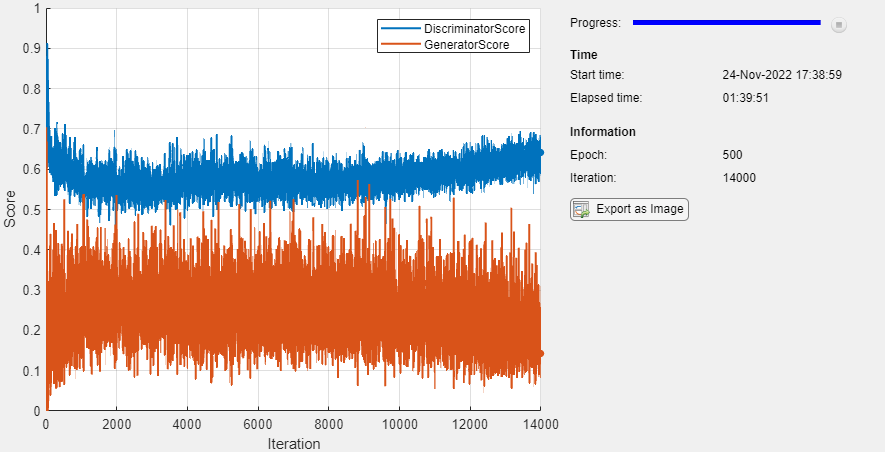
Here, the discriminator has learned a strong feature representation that identifies real images among generated images. In turn, the generator has learned a similarly strong feature representation that allows it to generate images similar to the training data.
The training plot shows the scores of the generator and discriminator networks. To learn more about how to interpret the network scores, see Monitor GAN Training Progress and Identify Common Failure Modes.
Generate New Images
To generate new images, use the predict function on the generator with a dlarray object containing a batch of random vectors. To display the images together, use the imtile function and rescale the images using the rescale function.
Create a dlarray object containing a batch of 25 random vectors to input to the generator network.
numObservations = 25;
ZNew = randn(numLatentInputs,numObservations,"single");
ZNew = dlarray(ZNew,"CB");
If a GPU is available, then convert the latent vectors to gpuArray.
if canUseGPU
    ZNew = gpuArray(ZNew);
end
Generate new images using the predict function with the generator and the input data.
XGeneratedNew = predict(netG,ZNew);
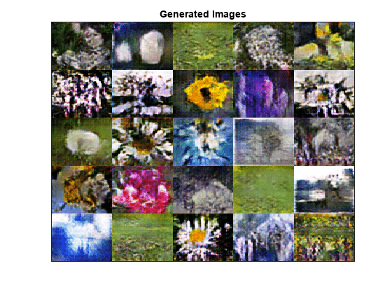
Display the images.
I = imtile(extractdata(XGeneratedNew));
I = rescale(I);
figure
image(I)
axis off
title("Generated Images")

Model Loss Function
The function modelLoss takes as input the generator and discriminator dlnetwork objects netG and netD, a mini-batch of input data X, an array of random values Z, and the probability to flip the real labels flipProb, and returns the loss values, the gradients of the loss values with respect to the learnable parameters in the networks, the generator state, and the scores of the two networks.
function [lossG,lossD,gradientsG,gradientsD,stateG,scoreG,scoreD] = ...
    modelLoss(netG,netD,X,Z,flipProb)

% Calculate the predictions for real data with the discriminator network.
YReal = forward(netD,X);

% Calculate the predictions for generated data with the discriminator
% network.
[XGenerated,stateG] = forward(netG,Z);
YGenerated = forward(netD,XGenerated);

% Calculate the score of the discriminator.
scoreD = (mean(YReal) + mean(1-YGenerated)) / 2;

% Calculate the score of the generator.
scoreG = mean(YGenerated);

% Randomly flip the labels of the real images.
numObservations = size(YReal,4);
idx = rand(1,numObservations) < flipProb;
YReal(:,:,:,idx) = 1 - YReal(:,:,:,idx);

% Calculate the GAN loss.
[lossG, lossD] = ganLoss(YReal,YGenerated);

% For each network, calculate the gradients with respect to the loss.
gradientsG = dlgradient(lossG,netG.Learnables,RetainData=true);
gradientsD = dlgradient(lossD,netD.Learnables);

end
GAN Loss Function and Scores
The objective of the generator is to generate data that the discriminator classifies as "real". To maximize the probability that images from the generator are classified as real by the discriminator, minimize the negative log likelihood function.
Given the output of the discriminator:
is the probability that the input image belongs to the class
"real".is the probability that the input image belongs to the class
"generated".
The loss function for the generator is given by
where contains the discriminator output probabilities for the generated images.
The objective of the discriminator is to not be "fooled" by the generator. To maximize the probability that the discriminator successfully discriminates between the real and generated images, minimize the sum of the corresponding negative log likelihood functions.
The loss function for the discriminator is given by
where contains the discriminator output probabilities for the real images.
To measure on a scale from 0 to 1 how well the generator and discriminator achieve their respective goals, you can use the concept of score.
The generator score is the average of the probabilities corresponding to the discriminator output for the generated images:
The discriminator score is the average of the probabilities corresponding to the discriminator output for both the real and generated images:
The score is inversely proportional to the loss but effectively contains the same information.
function [lossG,lossD] = ganLoss(YReal,YGenerated)

% Calculate the loss for the discriminator network.
lossD = -mean(log(YReal)) - mean(log(1-YGenerated));

% Calculate the loss for the generator network.
lossG = -mean(log(YGenerated));

end
Mini-Batch Preprocessing Function
The preprocessMiniBatch function preprocesses the data using the following steps:
Extract the image data from the incoming cell array and concatenate into a numeric array.
Rescale the images to be in the range
[-1,1].
function X = preprocessMiniBatch(data)

% Concatenate mini-batch
X = cat(4,data{:});

% Rescale the images in the range [-1 1].
X = rescale(X,-1,1,InputMin=0,InputMax=255);

end
References
The TensorFlow Team. Flowers http://download.tensorflow.org/example_images/flower_photos.tgz
Radford, Alec, Luke Metz, and Soumith Chintala. “Unsupervised Representation Learning with Deep Convolutional Generative Adversarial Networks.” Preprint, submitted November 19, 2015. http://arxiv.org/abs/1511.06434.
See Also
dlnetwork | forward | predict | dlarray | dlgradient | dlfeval | adamupdate | minibatchqueue
Topics
- Train Conditional Generative Adversarial Network (CGAN)
- Monitor GAN Training Progress and Identify Common Failure Modes
- Train Fast Style Transfer Network
- Generate Images Using Diffusion
- Custom Training Loops
- Train Network Using Custom Training Loop
- Specify Training Options in Custom Training Loop
- List of Deep Learning Layers