Denoise Signals with Generative Adversarial Networks
This example demonstrates how autoencoders (AEs) and generative adversarial networks (GANs) can be used for signal denoising. The example implements these deep learning models as objects that you can train using your own datasets of real, one-dimensional signals. You can then use the trained models to remove noise from signals similar to those used in the training.
The first part of the example trains the models to remove noise from synthetic sinusoidal signals corrupted with white Gaussian noise (WGN). The second and third parts of the example examine the efficacy of the models when denoising real-world noisy electrocardiogram (ECG) and seismic vibration signals.
Autoencoders
Autoencoders have been used in a wide variety of applications such as anomaly detection, image denoising, and sequence-to-sequence prediction. Autoencoders operate by first compressing the input to a lower-dimensional space called the latent space and then decompressing the latent space back into a space of higher dimensionality, typically one with the same size as the input. Autoencoders can be divided into two parts: the encoder which handles the compression, and the decoder which handles the decompression.
Generative Adversarial Networks
Generative adversarial networks have been widely used in image processing and are now being applied in other fields, including signal processing. A GAN comprises two submodels: a generator and a discriminator. The generator is typically the primary model of interest when training GANs. In this example, the generator is responsible for predicting the denoised signal from the noisy input. On the other hand, the discriminator is a supplementary model that you can leverage to improve the accuracy of the generator's predictions. This example uses as discriminator a binary classifier network that predicts whether the denoised signal produced by the generator is "real" (the true signal with zero noise) or "fake" (a prediction from the generator).
Case 1: Denoise Simple Sinusoids
This section demonstrates how to initialize and train the AE and GAN models and how to use the trained objects to denoise signals. The denoising performance is compared to an infinite-duration impulse response (IIR) lowpass filter.
Load and Visualize Data
The dataset contains simple sinusoidal signals corrupted with white Gaussian noise. Each signal consists of a sum of five sinusoidal components with random frequencies between 10 Hz and 256 Hz, random amplitudes between 0.5 and 5, and random initial phases phase between 0 and . Each signal is sampled at 1024 Hz for a random duration between 1 and 2 seconds and embedded in white noise such that the signal-to-noise ratio (SNR) is one of –5, –3, –1, 0, 2, 4, and 6 dB.
Generate the predictors, X, and targets, T, for the training, validation, and testing datasets. View the sizes of the datasets.
[X,T] = helperGenerateSines(50e3);
XTrain = X.Train;
TTrain = T.Train;
XValid = X.Valid;
TValid = T.Valid;
XTest = X.Test;
TTest = T.Test;
clear X T

whos XTrain TTrain XValid TValid
  Name            Size                Bytes  Class    Attributes

  TTrain      40000x1             495918840  cell
  TValid       5000x1              61968256  cell
  XTrain      40000x1             495918840  cell
  XValid       5000x1              61968256  cell
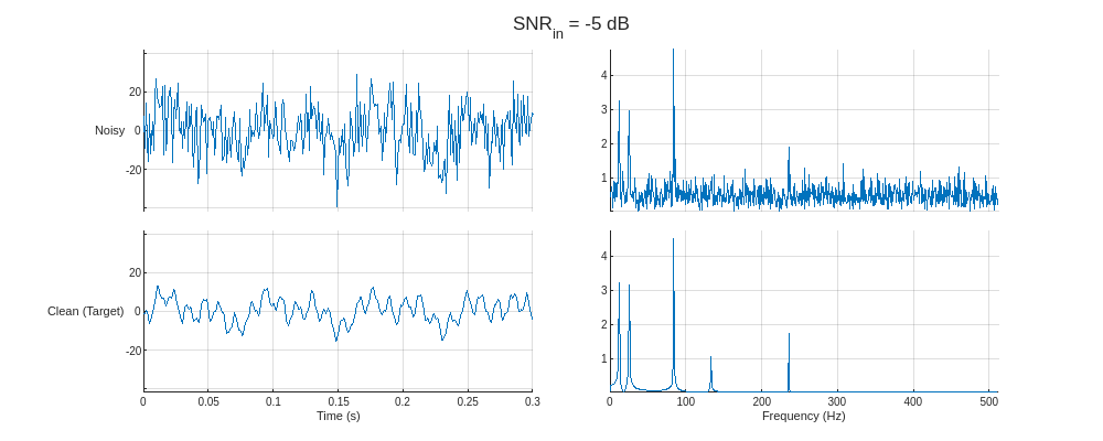
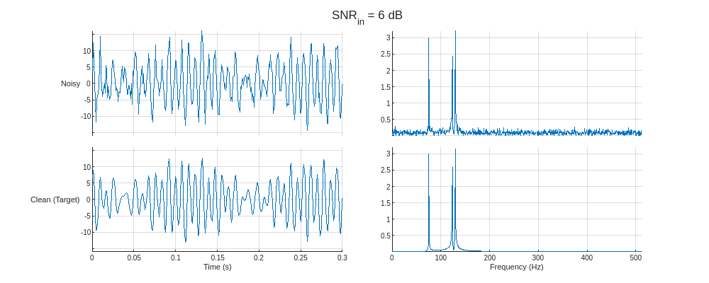
Plot the noisy predictor and clean target for the training signals with the lowest and highest SNR values. Display the time-domain signals and the corresponding one-sided spectra.
helperPlotTrainData(XTrain,TTrain,1024,true)
Create and Train Denoising Autoencoder
Create a helperDeepSignalDenoiserAE object and set its SignalLength property to 1024 based on the shortest possible length of the signals in the dataset. Set FilterSize to 128 for all convolutional layers. Set Leakiness to 0.3 for the leaky rectified linear unit (ReLU) layers, which can help when training on oscillating signals. Use the default values of 64 filters for each downsampling layer and 128 filters for each external layer. Use the default five downsampling layers to reduce the signal lengths to 32 in the latent space.
denoiserAESines = ...
    helperDeepSignalDenoiserAE(SignalLength=1024, ...
    FilterSize=128, ...
    Leakiness=0.3)
denoiserAESines =
  helperDeepSignalDenoiserAE with properties:

   State:
                    IsTrained: 0

   Network Options:
                 SignalLength: 1024
               NumDownSamples: 5
                   FilterSize: 128
    NumDownSampleLayerFilters: 64
      NumExternalLayerFilters: 128
                    Leakiness: 0.3000

   Model Architecture:
         DenoisingAutoencoder: [1×1 dlnetwork]

   Training Options/Results:
               TrainedNetwork: []
              TrainingOptions: []
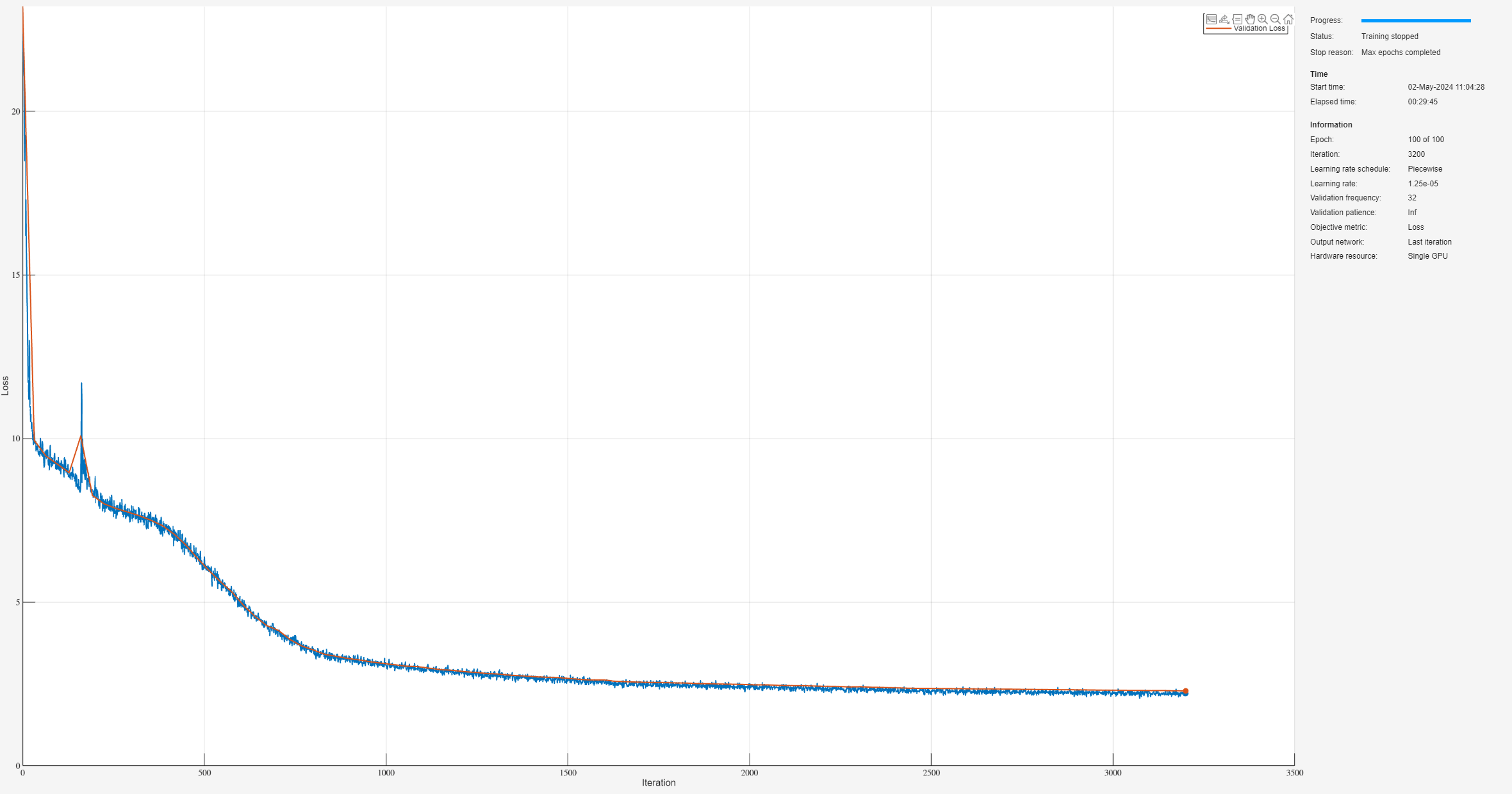
Define a structure array of training options. Use the default value of 1e-4 for the initial learn rate and a piecewise schedule to halve the learning rate every 25 epochs. Set the validation frequency to 32 iterations to perform validation at the end of each epoch. Set the doTrain flag to false to load a pretrained object instead of training.
doTrain =false; if doTrain trainOpts = ... struct(MaxEpochs=100, ... MiniBatchSize=1250, ... ValidationFrequency=32, ... LearnRateDropPeriod=25, ... LearnRateDropFactor=0.5); trainAE(denoiserAESines, ... [XTrain TTrain],[XValid TValid],trainOpts); else datasetZipFile = matlab.internal.examples.downloadSupportFile("SPT","data/trainedDenoiserObjectSines.zip"); datasetFolderSines = fullfile(fileparts(datasetZipFile),"trainedDenoiserObjectSines"); unzip(datasetZipFile,fileparts(datasetZipFile)); delete(datasetZipFile); load(fullfile(datasetFolderSines,"denoiserAESines.mat")) end
Create and Train Denoiser GAN
Create a helperDeepSignalDenoiserGAN object with the same properties as the denoising autoencoder.
denoiserGANSines = ...
    helperDeepSignalDenoiserGAN(SignalLength=1024, ...
    FilterSize=128, ...
    Leakiness=0.3)
denoiserGANSines =
  helperDeepSignalDenoiserGAN with properties:

   State:
                    IsTrained: 0

   Network Options:
                 SignalLength: 1024
               NumDownSamples: 5
                   FilterSize: 128
    NumDownSampleLayerFilters: 64
      NumExternalLayerFilters: 128
                    Leakiness: 0.3000

   Model Architectures:
                    Generator: [1×1 dlnetwork]
                Discriminator: [1×1 dlnetwork]

   Training Options/Results:
                  LastNetwork: []
    BestValidationLossNetwork: []
              TrainingOptions: []
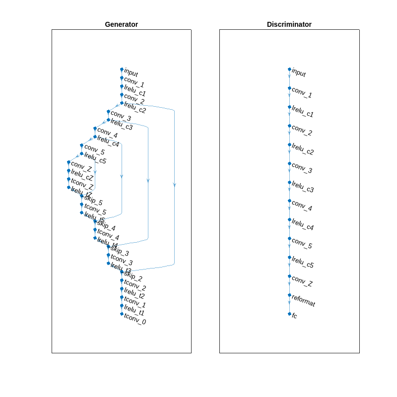
View the model architectures of the generator and discriminator networks. Because the same property values were used to initialize the GAN and the AE, the generator has the same architecture as the denoising AE. Additionally, the discriminator has the same architecture as the encoding portion of the denoising autoencoder, which is the first half containing the downsampling 1-D convolution layers.
helperPlotNetworks(denoiserGANSines)
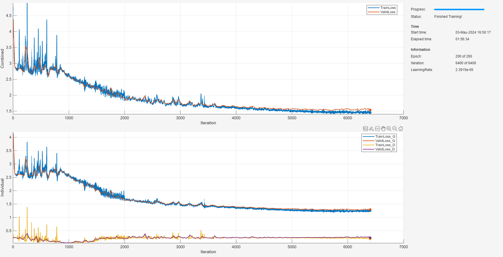
Define a structure array of training options. Set the initial learn rate to 5e-5, and use a piecewise learning rate schedule to reduce the learn rate by a factor of 0.9 every 25 epochs. Set the L1-norm loss factor to 0.001 when computing the generator's loss function to improve training efficacy. Set the validation frequency to 32 iterations to validate at the end of each epoch. Set the doTrain flag to false to load a pretrained object instead of training.
doTrain =false; if doTrain trainOpts = ... struct(MaxEpochs=200, ... MiniBatchSize=1250, ... ValidationFrequency=32, ... InitialLearnRate=5e-5, ... LearnRateDropPeriod=25, ... LearnRateDropFactor=0.9, ... L1LossFactor=0.001); trainGAN(denoiserGANSines, ... [XTrain TTrain],[XValid TValid],trainOpts); else load(fullfile(datasetFolderSines,"denoiserGANSines.mat")) end
Evaluate Denoising Performance
The signals used to train the object have SNRs ranging among –5, –3, –1, 0, 2, 4, and 6 dB. Compare the models' denoising performance with noisy signals with SNR values ranging from –7 to 7 dB.
Get denoised predictions for the testing data using the trained models.
YAE = denoise(denoiserAESines,XTest);
YGAN = denoise(denoiserGANSines,XTest);
Apply a lowpass IIR filter to the noisy data. Truncate the sequence lengths of the testing data to the SignalLength property defined for the denoising AE and GAN models. Generate the discrete-time filter object for a lowpass Butterworth filter with passband and stopband cuttoff frequencies of 256 Hz and 300 Hz, 0.05 dB passband ripple, and 60 dB stopband attenuation. Apply the lowpass filter to the testing data using a zero-phase digital filtering approach.
XTest = cellfun(@(X) X(1:denoiserGANSines.SignalLength), ...
    XTest,UniformOutput=false);
TTest = cellfun(@(T) T(1:denoiserGANSines.SignalLength), ...
    TTest,UniformOutput=false);

myFilter = designfilt("lowpassiir", ...
    DesignMethod="butter", ...
    SampleRate=1024, ...
    PassbandFrequency=256, ...
    StopbandFrequency=300, ...
    PassbandRipple=0.05, ...
    StopbandAttenuation=60);
YLP = cellfun(@(X) filtfilt(myFilter,X), ...
    XTest,UniformOutput=false);
Compute performance metrics: root mean squared error (RMSE), percent relative difference (PRD), and signal-to-noise ratio.
[RMSE_in,PRD_in,SNR_in] = helperComputeMetrics(XTest,TTest);
[RMSE_LP,PRD_LP,SNR_LP] = helperComputeMetrics(YLP,TTest);
[RMSE_AE,PRD_AE,SNR_AE] = helperComputeMetrics(YAE,TTest);
[RMSE_GAN,PRD_GAN,SNR_GAN] = helperComputeMetrics(YGAN,TTest);
Create box plots of the metrics to compare performance between the filter and the deep learning networks.
helperPlotMetrics([RMSE_in RMSE_LP RMSE_AE RMSE_GAN], ...
    [PRD_in PRD_LP PRD_AE PRD_GAN], ...
    [SNR_in SNR_LP SNR_AE SNR_GAN], ...
    ["Input" "LP" "AE" "GAN"])
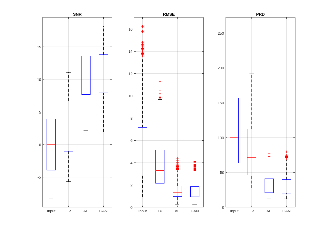
Both the autoencoder and GAN models produce denoised signals with notably higher SNRs and lower errors and relative differences than the lowpass filter. Although the GAN performs slightly better than the autoencoder, both deep learning models exhibit similar denoising performance overall.
Compare the denoising performance between the lowpass filter and the GAN model for the signals with the lowest and highest input SNR values.
helperCompareResults(XTest,TTest,YLP,YGAN,1024,["LP" "GAN"],true)
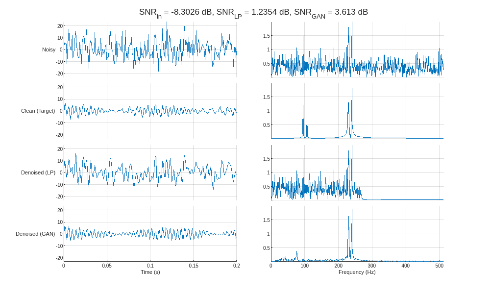
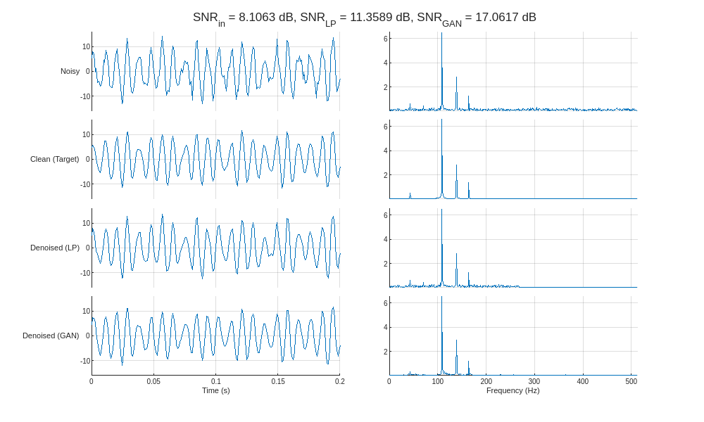
Inspecting the frequency spectra of the denoised signals reveals that the GAN removes noise in the frequency range between the component sinusoids, whereas the lowpass filter is only able to remove noise outside of the passband (above 256 Hz). In essence, the GAN behaves similarly to a multi-bandpass filter tuned specifically to the fundamental frequencies of each input signal.
Compute the average mean squared error (MSE) before and after denoising for each input SNR.
SNRs = -7:7;
MSE_in = zeros(length(SNRs),1);
MSE_LP = MSE_in;
MSE_AE = MSE_in;
MSE_GAN = MSE_in;

for ii = 1:length(SNRs)
    idx = find(round(SNR_in,1)-SNRs(ii) < 1);
    MSE_in(ii) = mean(RMSE_in(idx).^2);
    MSE_LP(ii) = mean(RMSE_LP(idx).^2);
    MSE_AE(ii) = mean(RMSE_AE(idx).^2);
    MSE_GAN(ii) = mean(RMSE_GAN(idx).^2);
end
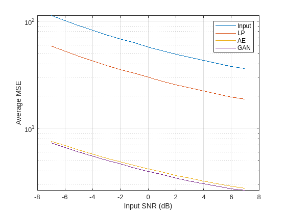
Plot the MSE as a function of input SNR for the noisy and denoised signals. The autoencoder and GAN produce denoised signals with significantly lower mean squared errors than those from the lowpass filter, likely due to their ability to remove noise between the fundamental frequencies of the sinusoids.
figure
semilogy(SNRs,[MSE_in MSE_LP MSE_AE MSE_GAN])
legend(["Input" "LP" "AE" "GAN"],Location="Northeast")
ylabel("Average MSE")
xlabel("Input SNR (dB)")
grid on
Case 2: Denoise ECG Signals
In this section, you train the autoencoder and generative adversarial network objects to denoise ECG signals and compare their generalization performance.
Load and Visualize Data
The dataset comprises real ECG signals and noise from the PhysioNet MIT-BIH Arrhythmia database [1][2] and MIT-BIH Noise Stress Test database [1][3]. All signals were sampled at 300 Hz and divided into 1024-sample segments. Three kinds of noise were used to corrupt the signals: baseline wander, muscle artifact, and electrode motion. The three are combined, rescaled to produce target SNRs of –2.5, 0, 2.5, 5, and 7.5 dB, and added to the clean signals.
Begin by loading the predictors and targets for both the training and validation datasets.
datasetZipFile = matlab.internal.examples.downloadSupportFile("SPT","data/PhysionetMITBIH.zip");
datasetFolderECG = fullfile(fileparts(datasetZipFile),"PhysionetMITBIH");
unzip(datasetZipFile,fileparts(datasetZipFile));
delete(datasetZipFile);
load(fullfile(datasetFolderECG,"ECG.mat"))
whos XTrain TTrain XValid TValid
  Name            Size                Bytes  Class    Attributes

  TTrain      38400x1             319180800  cell
  TValid       4800x1              39897600  cell
  XTrain      38400x1             319180800  cell
  XValid       4800x1              39897600  cell
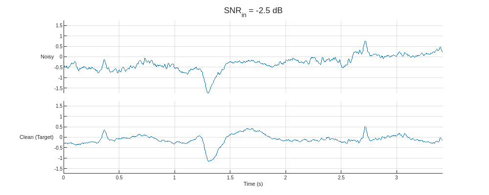
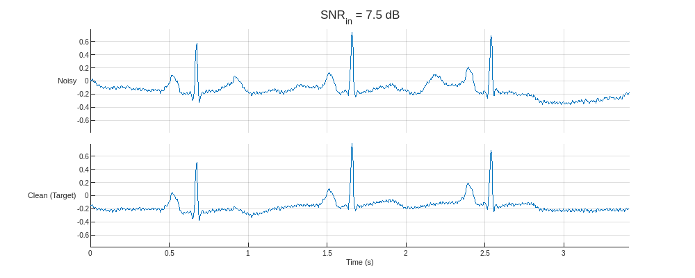
Plot the predictors from the training partition with the lowest and highest SNR and their corresponding clean targets.
helperPlotTrainData(XTrain,TTrain,300)
Create and Train Denoising Autoencoder
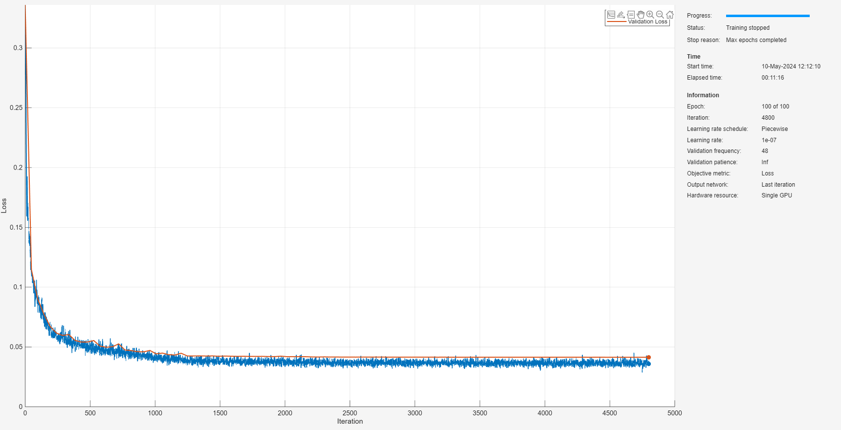
Train the denoising autoencoder model with the ECG data. Use default values for all model parameters. Configure the training loop to last 100 epochs and set the mini-batch size to 800, which equates to 48 mini-batches per epoch. Use an initial learn rate of 1e-4 and reduce the learn rate by half every 25 epochs. Set the doTrain flag to false to load a pretrained object instead of training.
doTrain =false; if doTrain denoiserAEECG = helperDeepSignalDenoiserAE() trainOpts = ... struct(MaxEpochs=100, ... MiniBatchSize=800, ... ValidationFrequency=48, ... LearnRateDropPeriod=25, ... LearnRateDropFactor=0.5); trainAE(denoiserAEECG, ... [XTrain TTrain],[XValid TValid],trainOpts); else datasetZipFile = matlab.internal.examples.downloadSupportFile("SPT","data/trainedDenoiserObjectECG.zip"); datasetFolderECG = fullfile(fileparts(datasetZipFile),"trainedDenoiserObjectECG"); unzip(datasetZipFile,fileparts(datasetZipFile)); delete(datasetZipFile); load(fullfile(datasetFolderECG,"denoiserAEECG.mat")) end
Create and Train Denoising GAN
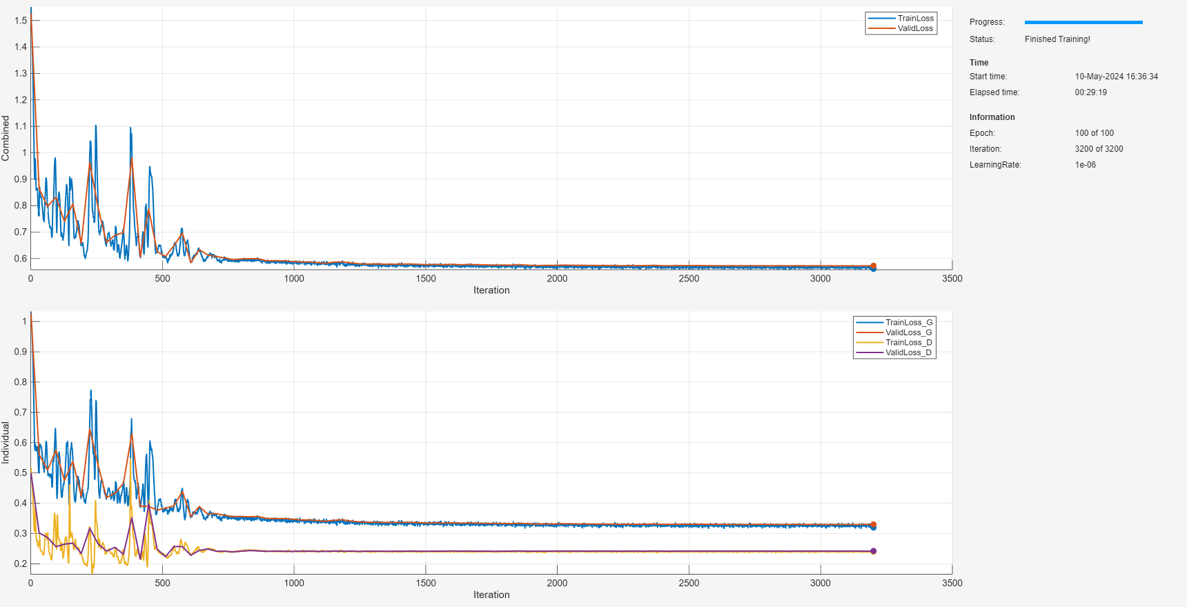
Train the denoising GAN model on the ECG data. Use the same architecture as the autoencoder by using default values for all model parameters. Set the maximum number of epochs to 200. Use a higher mini-batch size of 1200, which can sometimes help improve stability of the GAN training scheme. Use an initial learn rate of 1e-4 with a piecewise scheme that multiplies the learning rate by a reduction factor of every 40 epochs. Set the L1-norm loss factor to 0.05 when calculating the generator loss during training. Set the doTrain flag to false to load a pretrained object instead of training.
doTrain =false; if doTrain denoiserGANECG = helperDeepSignalDenoiserGAN() trainOpts = ... struct(MaxEpochs=200, ... MiniBatchSize=1200, ... ValidationFrequency=32, ... InitialLearnRate=1e-4, ... LearnRateDropPeriod=40, ... LearnRateDropFactor=sqrt(10)/10, ... L1LossFactor=0.05, ... OutputNetwork="both"); trainGAN(denoiserGANECG, ... [XTrain TTrain],[XValid TValid],trainOpts); else load(fullfile(datasetFolderECG,"denoiserGANECG.mat")) end
Compare Generalization Performance
Signals with slightly different characteristics were synthesized to test the generalization performance of the trained models. In this testing dataset, the signals were generated using the same procedure as for the training and validation sets; however, the testing signals have target SNRs of –1, 3, and 7 dB.
Load the noisy signals and clean targets for the testing partition from file.
whos XTess TTest
  Name          Size               Bytes  Class    Attributes

  TTest      2880x1             23938560  cell
Use the trained AE and GAN objects to denoise the testing data.
YAE = denoise(denoiserAEECG,XTest);
YGAN = denoise(denoiserGANECG,XTest);
Compute the performance metrics: RMSE, PRD, and SNR.
[RMSE_in,PRD_in,SNR_in] = helperComputeMetrics(XTest,TTest);
[RMSE_AE,PRD_AE,SNR_AE] = helperComputeMetrics(YAE,TTest);
[RMSE_GAN,PRD_GAN,SNR_GAN] = helperComputeMetrics(YGAN,TTest);
Compare the overall denoising results using box plots.
helperPlotMetrics([RMSE_in RMSE_AE RMSE_GAN], ...
    [PRD_in PRD_AE PRD_GAN], ...
    [SNR_in SNR_AE SNR_GAN], ...
    ["Input" "AE" "GAN"])
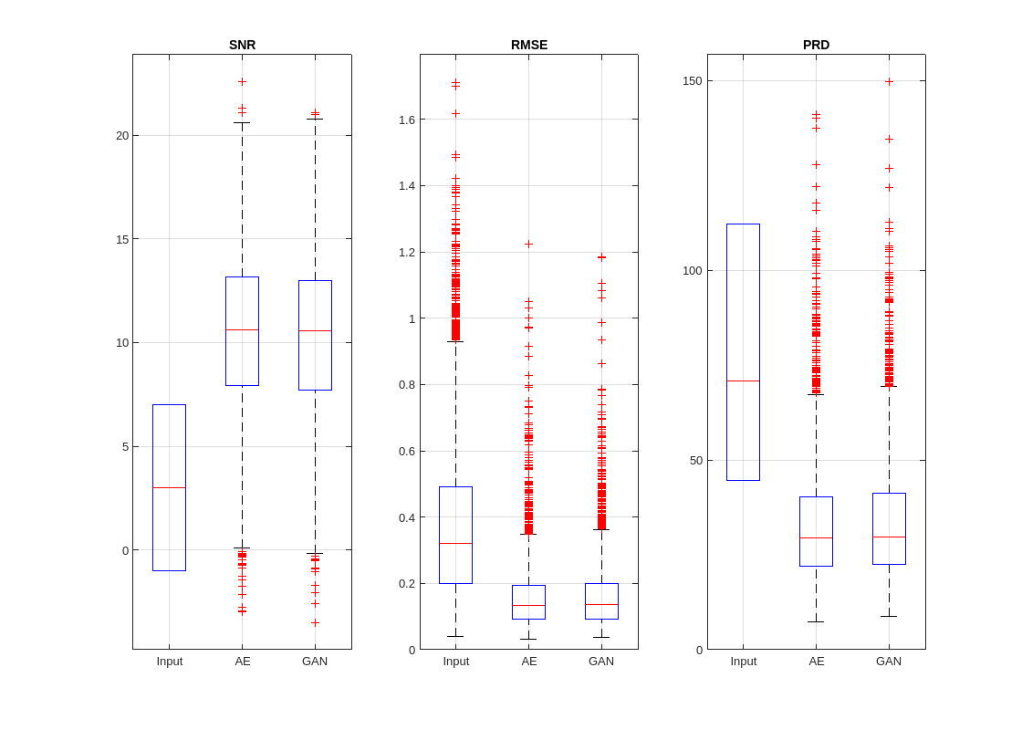
The autoencoder and GAN exhibit similar denoising performance overall. However, the autoencoder is slightly better at producing signals with higher SNR and lower error on average.
Plot the results (prediction) alongside the noisy signal (predictor) and clean signal (target) for the highest and lowest input SNR.
helperCompareResults(XTest,TTest,YAE,YGAN,300)
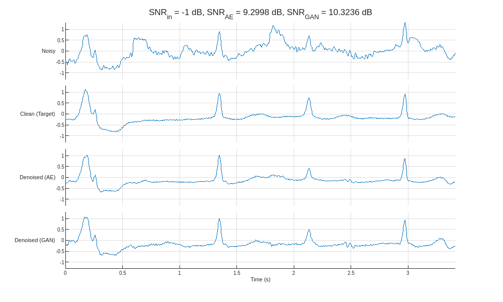
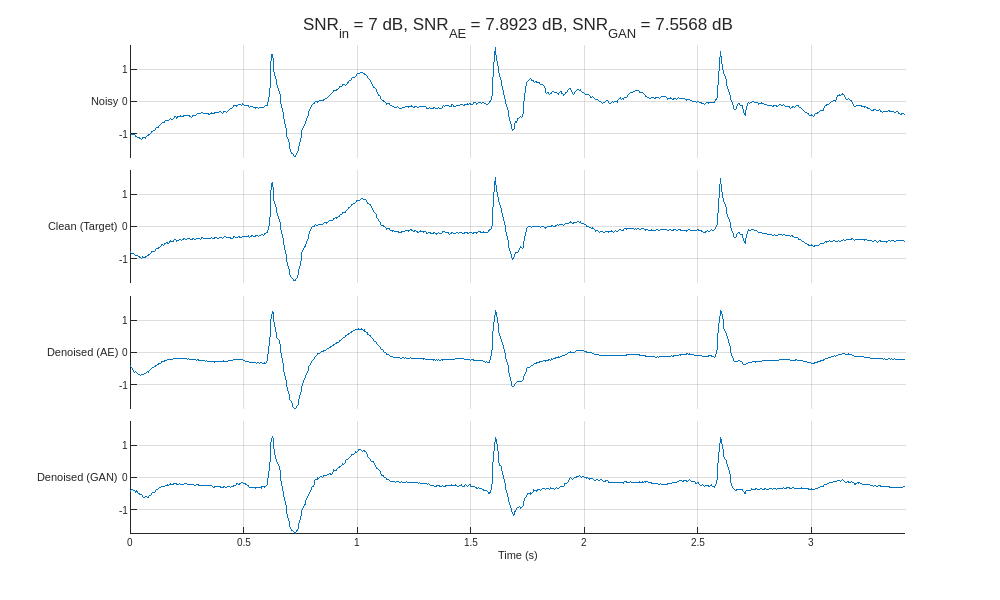
Compared to the autoencoder, the GAN produces denoised signals with peak amplitudes closer to the clean target. Close inspection of the denoised signals reveals that the autoencoder exhibits a smoothing phenomenon that is effective at removing noise but results in less accurate peak shapes and amplitudes.
Compute the average MSE before and after denoising for each input SNR.
SNRs = -1:4:7;
MSE_in = zeros(length(SNRs),1);
MSE_AE = MSE_in;
MSE_GAN = MSE_in;

for ii = 1:length(SNRs)
    idx = find(round(SNR_in,1)-SNRs(ii) < 1);
    MSE_in(ii) = mean(RMSE_in(idx).^2);
    MSE_AE(ii) = mean(RMSE_AE(idx).^2);
    MSE_GAN(ii) = mean(RMSE_GAN(idx).^2);
end
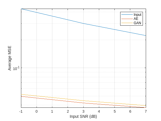
Plot the MSE as a function of input SNR for the noisy and denoised signals. The autoencoder and GAN both generate denoised signals with notably lower mean squared errors than the noisy inputs. However, the autoencoder consistently produces signals with slightly lower MSE.
figure
semilogy(SNRs,[MSE_in MSE_AE MSE_GAN])
legend(["Input" "AE" "GAN"],Location="Northeast")
ylabel("Average MSE")
xlabel("Input SNR (dB)")
grid on
Case 3: Denoise Seismic Vibration Signals
In this section, you train the denoising autoencoder and generative adversarial network objects on earthquake measurements and compare their denoising performance.
Load and Visualize Data
This section uses a preprocessed version of the Stanford Earthquake Dataset (STEAD) [4]. The subset used is constructed by randomly selecting 20,000 seismic measurements of 60-second durations sampled at 100 Hz and individually normalizing them based on their maximum amplitudes. The noise data are constructed from a basis of 2907 entries of isolated noise that are also randomly sampled and rescaled to achieve target SNRs of –10, –6, –2, 2, and 6 dB with respect to the seismic signals. Finally, the signals are separated into the training, validation, and testing sets using an 80–10–10 split.
Load the predictors and targets for both the training and validation datasets.
datasetZipFile = matlab.internal.examples.downloadSupportFile("SPT","data/STEAD.zip");
datasetFolderSeismic = fullfile(fileparts(datasetZipFile),"STEAD");
unzip(datasetZipFile,fileparts(datasetZipFile));
delete(datasetZipFile);
load(fullfile(datasetFolderSeismic,"Earthquake.mat"))
whos XTrain TTrain XValid TValid
  Name            Size                Bytes  Class    Attributes

  TTrain      16000x1             526208000  cell
  TValid       2000x1              65776000  cell
  XTrain      16000x1             526208000  cell
  XValid       2000x1              65776000  cell
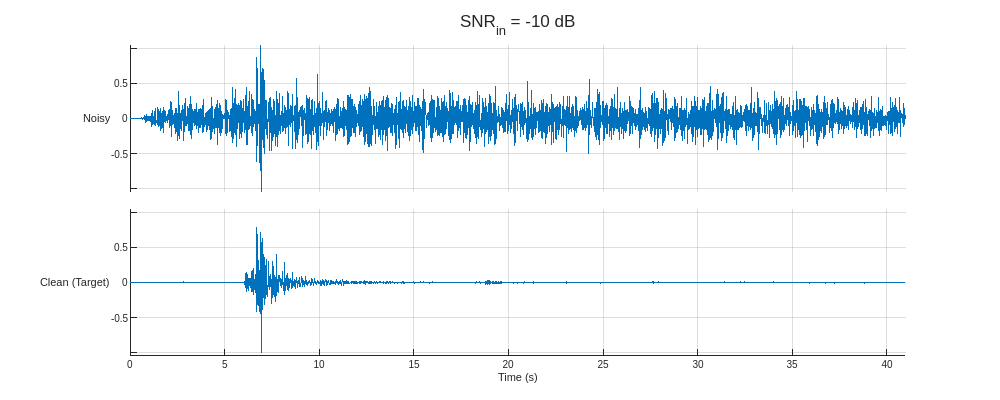
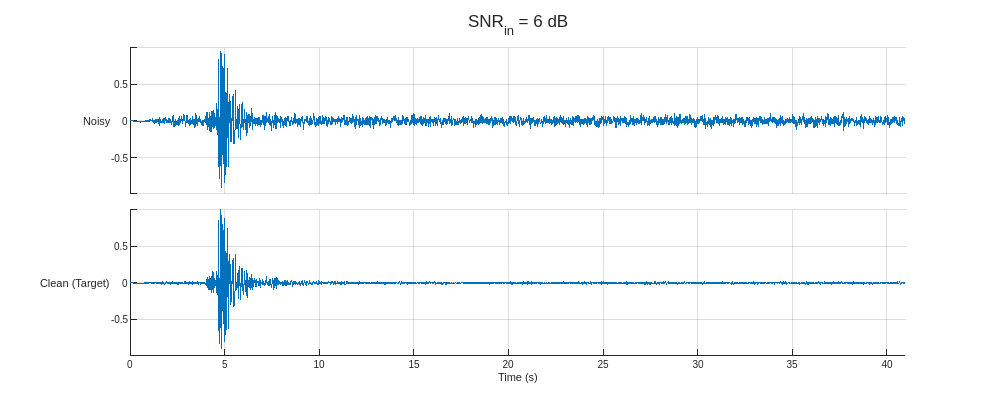
Plot the predictors from the training partition with the lowest and highest SNR and their corresponding clean targets.
helperPlotTrainData(XTrain,TTrain,100)
Create and Train Denoising Autoencoder
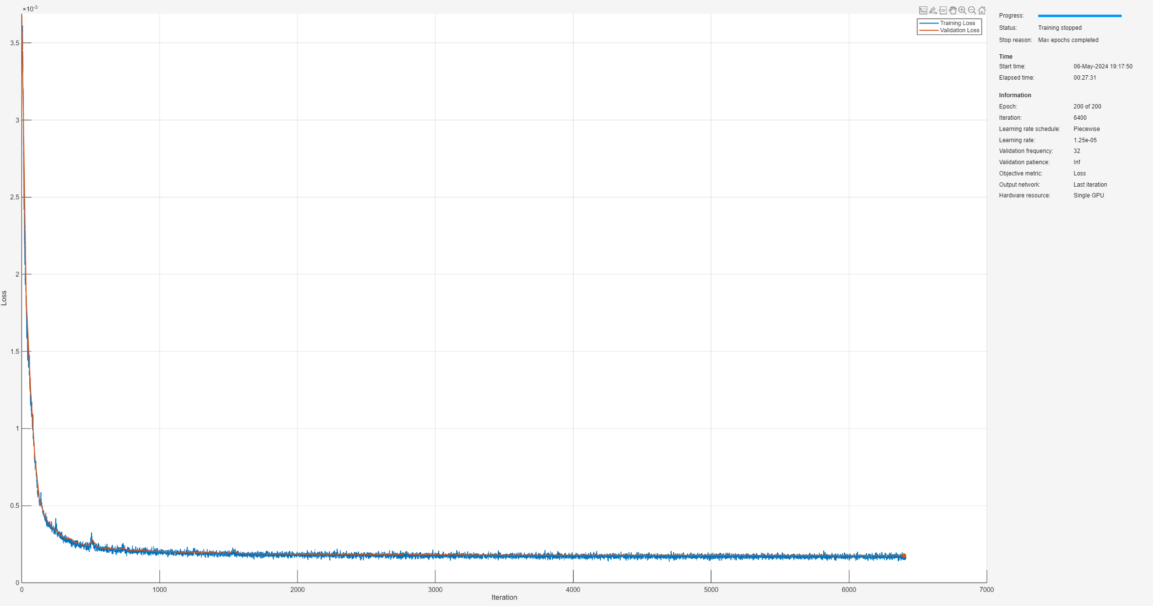
Train the autoencoder model with the seismic data. Set the autoencoder to a signal length of 4096 with four downsampling layers, 64 and 32 filters for the external and internal convolutional layers, a convolutional filter size of 64, and use 0.1 for the leakiness of the leaky ReLU layers. Set the training duration to 200 epochs and set the mini-batch size to 500 to achieve 32 mini-batches per epoch. Use an initial learn rate of 1e-4, and use a piecewise learning scheme to halve it every 50 epochs. Set the validation frequency to 32 to perform validation at the end of every epoch. Set the doTrain flag to false to load a pretrained object instead of training.
doTrain =false; if doTrain denoiserAESeismic = ... helperDeepSignalDenoiserAE(SignalLength=4096, ... NumDownSamples=4, ... FilterSize=64, ... NumDownSampleLayerFilters=32, ... NumExternalLayerFilters=64, ... Leakiness=0.1) trainOpts = struct(MaxEpochs=200, ... MiniBatchSize=500, ... ValidationFrequency=32, ... LearnRateDropPeriod=50, ... LearnRateDropFactor=0.5); trainAE(denoiserAESeismic, ... [XTrain TTrain],[XValid TValid],trainOpts); else datasetZipFile = matlab.internal.examples.downloadSupportFile("SPT","data/trainedDenoiserObjectSeismic.zip"); datasetFolderECG = fullfile(fileparts(datasetZipFile),"trainedDenoiserObjectSeismic"); unzip(datasetZipFile,fileparts(datasetZipFile)); delete(datasetZipFile); load(fullfile(datasetFolderECG,"denoiserAESeismic.mat")) end
Create and Train Denoising GAN
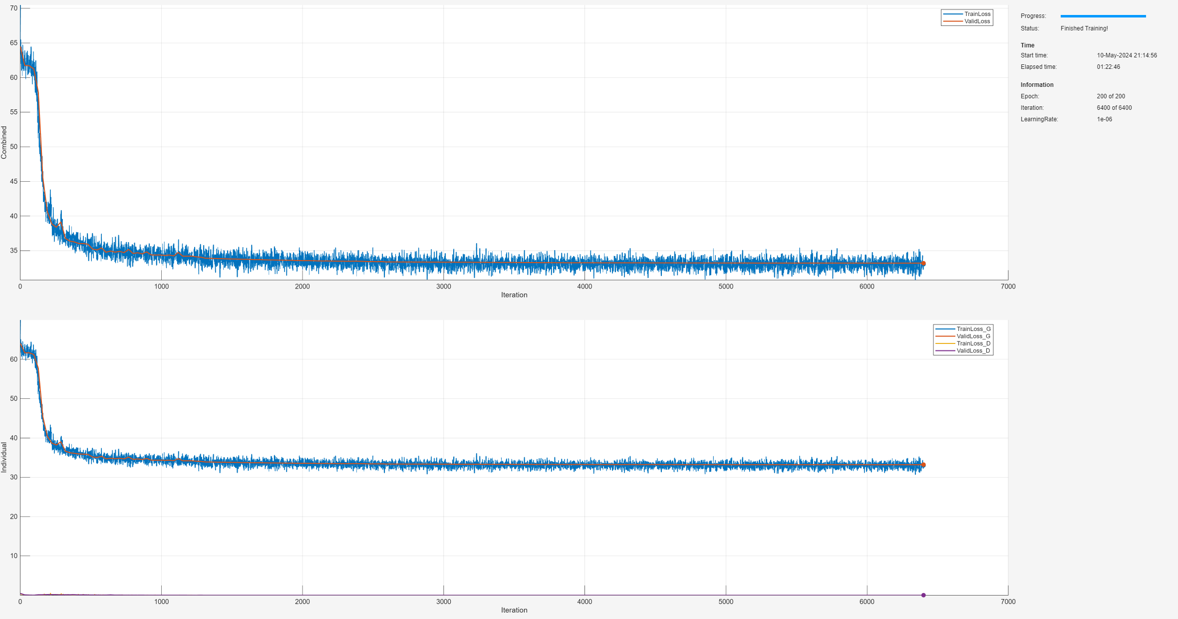
Train the denoising GAN model for seismic signal denoising. Configure the training loop to terminate after 200 epochs and set the mini-batch size to 500. Set 1e-4 as the initial learn rate. Use a piecewise learning scheme to multiply the learn rate by a reduction factor of 0.9 every 10 epochs. Set L1LossFactor to 1 to use the L1-norm of residual errors when computing the generator's loss. The GradientDecay factor is set to 0.5 for the GAN (compared to 0.9 when training the AE), which can help improve the stability of training. Set the doTrain flag to false to load a pretrained object instead of training.
doTrain =false; if doTrain denoiserGANSeismic = ... helperDeepSignalDenoiserGAN(SignalLength=4096, ... NumDownSamples=4, ... FilterSize=64, ... NumDownSampleLayerFilters=32, ... NumExternalLayerFilters=64, ... Leakiness=0.1) trainOpts = struct(MaxEpochs=200, ... MiniBatchSize=500, ... ValidationFrequency=32, ... InitialLearnRate=1e-4, ... LearnRateDropPeriod=10, ... LearnRateDropFactor=0.9, ... L1LossFactor=1, ... GradientDecay=0.5, ... OutputNetwork="both"); trainGAN(denoiserGANSeismic, ... [XTrain TTrain],[XValid TValid],trainOpts); else load(fullfile(datasetFolderECG,"denoiserGANSeismic.mat")) end
Compare Generalization Performance
The testing signals are created with slightly different characteristics to test the generalization performance of the trained objects. The signals in the testing partition were generated using the same procedure as for the training and validation partitions but with target SNRs ranging between –12 and 8 dB with increments of 2 dB.
Load the noisy signals and clean targets for the testing partition from file.
whos XTest TTest
  Name          Size               Bytes  Class    Attributes

  TTest      2000x1             65776000  cell
  XTest      2000x1             65776000  cell
Use the trained AE and GAN objects to denoise the testing data.
YAE = denoise(denoiserAESeismic,XTest);
YGAN = denoise(denoiserGANSeismic,XTest);
Compute the RMSE, PRD, and SNR metrics.
[RMSE_in,PRD_in,SNR_in] = helperComputeMetrics(XTest,TTest);
[RMSE_AE,PRD_AE,SNR_AE] = helperComputeMetrics(YAE,TTest);
[RMSE_GAN,PRD_GAN,SNR_GAN] = helperComputeMetrics(YGAN,TTest);
Compare the overall denoising performance using box plots.
helperPlotMetrics([RMSE_in RMSE_AE RMSE_GAN], ...
    [PRD_in PRD_AE PRD_GAN], ...
    [SNR_in SNR_AE SNR_GAN], ...
    ["Input" "AE" "GAN"])
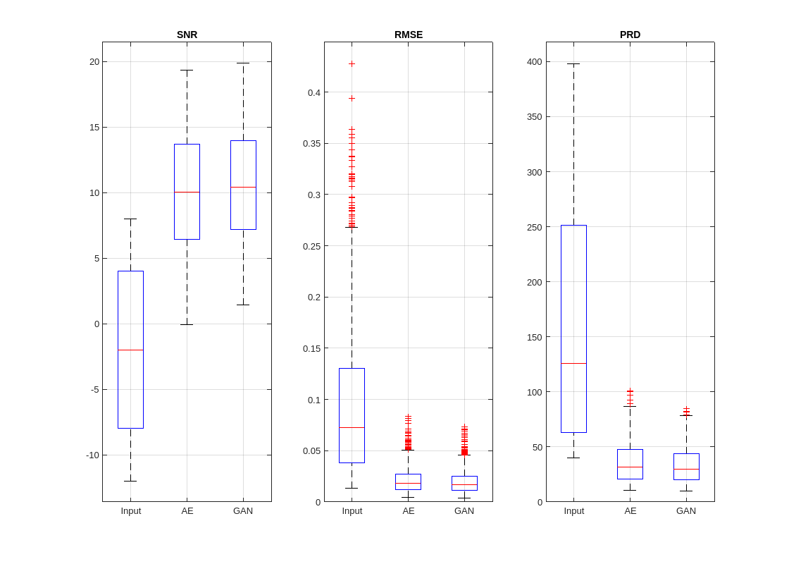
The GAN slightly outperforms the AE at improving SNR and reducing the RMSE and PRD of the signals in the test partition. However, both deep learning models are able to produce denoised signals with significantly higher SNRs compared to the noisy input signals.
Plot the best and worst denoised results (prediction) alongside the noisy signal (predictor) and clean signal (target).
helperCompareResults(XTest,TTest,YAE,YGAN,100)

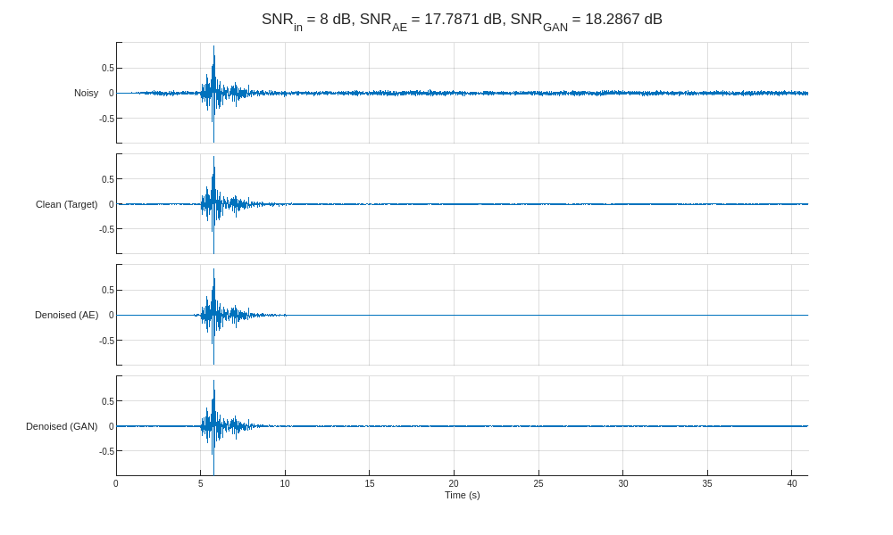
The GAN generates slightly more accurate denoised signals than the autoencoder. Most notably, however, both models demonstrate the ability to identify the approximate onset of seismic activity for input signals with significantly low SNR.
Compute the average MSE before and after denoising for each input SNR.
SNRs = -12:2:8;
MSE_in = zeros(length(SNRs),1);
MSE_AE = MSE_in;
MSE_GAN = MSE_in;

for ii = 1:length(SNRs)
    idx = find(round(SNR_in,1)-SNRs(ii) < 1);
    MSE_in(ii) = mean(RMSE_in(idx).^2);
    MSE_AE(ii) = mean(RMSE_AE(idx).^2);
    MSE_GAN(ii) = mean(RMSE_GAN(idx).^2);
end
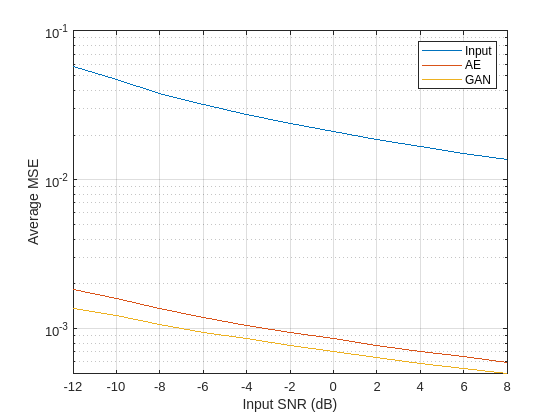
Plot the results to compare the MSE of the denoised signals produced by the AE and GAN models for each input SNR. The GAN produces denoised signals with lower average mean squared error than the autoencoder for all input SNR values. However, both deep learning models reduce the average MSE of the noisy inputs by more than an order of magnitude.
figure
semilogy(SNRs,[MSE_in MSE_AE MSE_GAN])
legend(["Input" "AE" "GAN"],Location="Northeast")
ylabel("Average MSE")
xlabel("Input SNR (dB)")
grid on
Conclusion
This example shows how to train autoencoder and generative adversarial deep learning networks to remove noise from different types of signals. Both model types are provided as custom MATLAB® classes via M-files, and they can be immediately used to train on your own dataset of one-dimensional signals. In the examples shown here, GAN tends to have slightly better performance than the AE. However, the GAN is more expensive to train with regard to time and computational cost. It is good practice to train and compare the two models to see which one works best for a particular set of data.
Acknowledgment
This example contains information from the PhysioNet MIT-BIH Arrhythmia Database and the PhysioNet MIT-BIH Noise Stress Test Database, which are made available under the Open Data Commons Attribution License (ODC-By) v1.0 available at https://opendatacommons.org/licenses/by/1-0/.
This example contains information from the STanford EArthquake Dataset (STEAD), which is made available under the Creative Commons Attribution License v4.0 International available at https://creativecommons.org/licenses/by/4.0/. The MathWorks, Inc. makes no warranty of any kind, express or implied, regarding the accuracy, validity, reliability, availability, or completeness of any information derived from this dataset. Copyright © 2019 S. Mostafa Mousavi, Yixiao Sheng, Weiqiang Zhu, and Gregory C. Beroza.
References
[1] Goldberger, A., L. Amaral, L. Glass, J. Hausdorff, P. C. Ivanov, R. Mark, J. E. Mietus, G. B. Moody, C. K. Peng, and H. E. Stanley. "PhysioBank, PhysioToolkit, and PhysioNet: Components of a new research resource for complex physiologic signals. Circulation [Online]. 101 (23), pp. e215–e220. (2000).
[2] Moody, G. B., and R. G. Mark. "The impact of the MIT-BIH Arrhythmia Database." IEEE Engineering in Medicine and Biology Magazine, vol. 20, no. 3, pp.45–50, May–June 2001. (PMID: 11446209)
[3] Moody, G. B., W. E. Muldrow, and R. G. Mark. "A noise stress test for arrhythmia detectors." Computers in Cardiology, vol. 11, pp. 381–384, 1984.
[4] Mousavi, S. M., Y. Sheng, W. Zhu, and G. C. Beroza. "STanford EArthquake Dataset (STEAD): A Global Data Set of Seismic Signals for AI." IEEE Access, vol. 7, pp. 179464–76, 2019. https://doi.org/10.1109/ACCESS.2019.2947848.
Appendix: Helper Functions
helperPlotNetworks
This function plots the architecture of the generator and discriminator networks of an input helperDeepSignalDenoiserGAN object.
function helperPlotNetworks(obj)
% This function is only intended to support this example.
% It may be changed or removed in a future release.

figure(Position=[0 0 1000 1000])
tiledlayout(1,2,TileSpacing="compact")
nexttile
plot(obj.Generator)
title("Generator")
nexttile
plot(obj.Discriminator)
title("Discriminator")

end
helperPlotTrainData
This function plots the input and target signals from the training partition with the highest and lowest SNR values.
function helperPlotTrainData(X,T,fsample,plotFreqSpectrum)
% This function is only intended to support this example.
% It may be changed or removed in a future release.

% Setup for potential subplotting
if nargin < 4
    plotFreqSpectrum = 0;
    tileFactor = 0;
elseif plotFreqSpectrum > 0
    tileFactor = 1;
end

% Identify highest and lowest SNR inputs
SNRs = cellfun(@(x,t) snr(t,x-t), X, T);
[val(1),ind(1)] = min(SNRs);
[val(2),ind(2)] = max(SNRs);

% Plot examples via loop
for ii = 1:2
    % Initialize plot
    figure(Position=[0 0 1000 400])
    tl = tiledlayout(1,tileFactor+1,TileSpacing="compact");
    tl.Title.String = "SNR_{in} = "+val(ii)+" dB";

    % Time domain plots
        % Prepare to transpose if necessary
        [nRow,nCol] = size(X{1});

        % Compute time domain and get signals
        L = length(X{ind(ii)});
        time = linspace(0,L/fsample,L);
        if nRow > nCol
            X_time = X{ind(ii)};
            T_time = T{ind(ii)};
        else
            X_time = X{ind(ii)}';
            T_time = T{ind(ii)}';
        end

        % Plot predictor and target (time domain)
        nexttile(tl,1)
        ax = stackedplot(time,[X_time T_time]);
        ax.DisplayLabels = ["Noisy" "Clean (Target)"];
        lims = [min(ax.AxesProperties(1).YLimits(1), ...
            ax.AxesProperties(2).YLimits(1)) ...
            max(ax.AxesProperties(1).YLimits(2), ...
            ax.AxesProperties(2).YLimits(2))];
        lims = max(abs(lims)).*[-1 1];
        [ax.AxesProperties(1).YLimits, ...
            ax.AxesProperties(2).YLimits] = deal(lims);
        ax.XLabel = "Time (s)";
        grid on

    % Frequency domain plots, if requested
    if plotFreqSpectrum
        % First, zoom the time domain plots
        ax.XLimits = [0 round(time(floor(end/5)),1)];

        % Single-sided FFT for predictor and target
        freq = fsample*(0:floor(L/2))/L;
        X_freq = fft(X_time);
        X_freq = abs(X_freq(1:floor(L/2)+1))/L;
        X_freq(2:end-1) = 2*X_freq(2:end-1);
        T_freq = fft(T_time);
        T_freq = abs(T_freq(1:floor(L/2)+1))/L;
        T_freq(2:end-1) = 2*T_freq(2:end-1);

        % Plot predictor and target (freq domain)
        nexttile(tl,2)
        ax = stackedplot(freq,[X_freq T_freq]);
        ax.DisplayLabels = ["" ""];
        lims = [min(ax.AxesProperties(1).YLimits(1), ...
            ax.AxesProperties(2).YLimits(1)) ...
            max(ax.AxesProperties(1).YLimits(2), ...
            ax.AxesProperties(2).YLimits(2))];
        lims = [0 max(abs(lims))];
        [ax.AxesProperties(1).YLimits, ...
            ax.AxesProperties(2).YLimits] = deal(lims);
        ax.XLimits = [0 round(freq(end))];
        ax.XLabel = "Frequency (Hz)";
        grid on

    end
end

end
helperCompareResults
This function plots two denoised signals alongside the input and target signals.
function helperCompareResults(X,T,Y1,Y2,fsample,modelLabels, ...
    plotFreqSpectrum)
% This function is only intended to support this example.
% It may be changed or removed in a future release.

% Setup based on number of input arguments
if nargin < 7
    plotFreqSpectrum = 0;
    tileFactor = 0;
elseif plotFreqSpectrum > 0
    tileFactor = 1;
end
if nargin < 6
    modelLabels = ["AE" "GAN"];
end

% Identify highest and lowest SNR inputs
SNRs = cellfun(@(x,t) snr(t,x-t),X,T);
[val(1),ind(1)] = min(SNRs);
[val(2),ind(2)] = max(SNRs);

% Plot examples via loop
for ii = 1:2
    % Prepare to transpose if necessary
    [nRow,nCol] = size(X{1});

    % Get signals, and compute prediction SNRs
    if nRow > nCol
        X_time = X{ind(ii)};
        T_time = T{ind(ii)};
        Y1_time = Y1{ind(ii)};
        Y2_time = Y2{ind(ii)};
    else
        X_time = X{ind(ii)}';
        T_time = T{ind(ii)}';
        Y1_time = Y1{ind(ii)}';
        Y2_time = Y2{ind(ii)}';
    end
    SNR_out1 = snr(Y1_time,Y1_time-T_time);
    SNR_out2 = snr(Y2_time,Y2_time-T_time);

    % Initialize plot
    figure(Position=[0 0 1000 600])
    tl = tiledlayout(1,tileFactor+1,TileSpacing="compact");
    tl.Title.String = "SNR_{in} = "+val(ii)+" dB, "+ ...
        "SNR_{"+modelLabels(1)+"} = "+SNR_out1+" dB, "+ ...
        "SNR_{"+modelLabels(2)+"} = "+SNR_out2+" dB";

    % Time domain plots
        % Compute time domain
        L = length(X{ind(ii)});
        time = linspace(0,L/fsample,L);

        % Plot predictor, target, and prediction (time domain)
        nexttile(tl,1)
        ax = stackedplot(time,[X_time T_time Y1_time Y2_time]);
        ax.DisplayLabels = ["Noisy" "Clean (Target)" ...
           "Denoised ("+modelLabels(1)+")" ...
           "Denoised ("+modelLabels(2)+")"];
        lims = [min([ax.AxesProperties(1).YLimits(1) ...
            ax.AxesProperties(2).YLimits(1) ...
            ax.AxesProperties(3).YLimits(1) ...
            ax.AxesProperties(4).YLimits(1)]) ...
            max([ax.AxesProperties(1).YLimits(2) ...
            ax.AxesProperties(2).YLimits(2) ...
            ax.AxesProperties(3).YLimits(2) ...
            ax.AxesProperties(4).YLimits(2)])];
        lims = max(abs(lims)).*[-1 1];
        [ax.AxesProperties(1).YLimits, ...
            ax.AxesProperties(2).YLimits, ...
            ax.AxesProperties(3).YLimits, ...
            ax.AxesProperties(4).YLimits] = deal(lims);
        ax.XLabel = "Time (s)";
        grid on

    % Frequency domain plots, if requested
    if plotFreqSpectrum
        % First, zoom the time domain plots
        ax.XLimits = [0 round(time(floor(end/5)),1)];

        % Single-sided FFT for predictor, target, and predictions
        freq = fsample*(0:(L/2))/L;
        X_freq = fft(X_time);
        X_freq = abs(X_freq(1:L/2+1))/L;
        X_freq(2:end-1) = 2*X_freq(2:end-1);
        T_freq = fft(T_time);
        T_freq = abs(T_freq(1:L/2+1))/L;
        T_freq(2:end-1) = 2*T_freq(2:end-1);
        Y1_freq = fft(Y1_time);
        Y1_freq = abs(Y1_freq(1:L/2+1))/L;
        Y1_freq(2:end-1) = 2*Y1_freq(2:end-1);
        Y2_freq = fft(Y2_time);
        Y2_freq = abs(Y2_freq(1:L/2+1))/L;
        Y2_freq(2:end-1) = 2*Y2_freq(2:end-1);

        % Plot predictor, target, and prediction (freq domain)
        nexttile(tl,2)
        ax = stackedplot(freq,[X_freq T_freq Y1_freq Y2_freq]);
        ax.DisplayLabels = ["" "" "" ""];
        lims = [min([ax.AxesProperties(1).YLimits(1) ...
            ax.AxesProperties(2).YLimits(1) ...
            ax.AxesProperties(3).YLimits(1) ...
            ax.AxesProperties(4).YLimits(1)]) ...
            max([ax.AxesProperties(1).YLimits(2) ...
            ax.AxesProperties(2).YLimits(2) ...
            ax.AxesProperties(3).YLimits(2) ...
            ax.AxesProperties(4).YLimits(2)])];
        lims = max(abs(lims)).*[0 1];
        [ax.AxesProperties(1).YLimits, ...
            ax.AxesProperties(2).YLimits, ...
            ax.AxesProperties(3).YLimits, ...
            ax.AxesProperties(4).YLimits] = deal(lims);
        ax.XLimits = [0 round(freq(end))];
        ax.XLabel = "Frequency (Hz)";
        grid on

    end
end

end
helperComputeMetrics
This function computes the RMSE, PRD, and SNR performance metrics.
function [RMSE,PRD,SNR] = helperComputeMetrics(Y,T)
% This function is only intended to support this example.
% It may be changed or removed in a future release.

RMSE = cellfun(@(Y,T) rmse(Y,T),Y,T,UniformOutput=true);

PRD = cellfun(@(Y,T) 100*sqrt(sum((Y-T).^2)./sum(T.^2)), ...
    Y,T,UniformOutput=true);

SNR = cellfun(@(Y,T) snr(T,Y-T),Y,T,UniformOutput=true);

end
helperPlotMetrics
This function plots the RMSE, PRD, and SNR performance metrics.
function helperPlotMetrics(RMSE,PRD,SNR,labels)
% This function is only intended to support this example.
% It may be changed or removed in a future release.

figure(Position=[0 0 1400 1000])
subplot(1,3,1)
    boxplot(SNR)
    title("SNR")
    xticklabels(labels)
    grid on
spax = subplot(1,3,2);
    boxplot(RMSE)
    title("RMSE")
    xticklabels(labels)
    grid on
    spax.YLim(1) = 0;
spax = subplot(1,3,3);
    boxplot(PRD)
    title("PRD")
    xticklabels(labels)
    grid on
    spax.YLim(1) = 0;

end
helperGenerateSines
This function generates training and testing sets of simple sinusoidal signals with added Gaussian white noise.
function [X,T] = helperGenerateSines(numSignals)
% This function is only intended to support this example.
% It may be changed or removed in a future release.

% Specify train/valid/test partitioning
partSizes = [80 10 10]./100;
partNames = ["Train" "Valid" "Test"];

% Specify signal characteristics
seqLength = [1024 2048];  % Range of sequence lengths to consider
magRange = [0.5 5];       % Range of magnitudes
freqRange = [10 256];     % Range of frequencies (Hz)
numSinesPerSig = 5;       % Number of component sinusoids per signal

% Define SNR targets for each partition
SNR_targ.Train = [-5 -3 -1 0 2 4 6];
SNR_targ.Valid = [-5 -3 -1 0 2 4 6];
SNR_targ.Test  = -7:7;

% Define time domain
t = linspace(0,seqLength(2)/seqLength(1), ...
    seqLength(2));

% Loop over number of partitions
for ii = 1:length(partSizes)
    % Initialize arrays for T and N
    if ii == 1
        T.(partNames(ii)) = ...
            zeros(ceil(partSizes(ii)*numSignals),seqLength(2));
    else
        T.(partNames(ii)) = ...
            zeros(floor(partSizes(ii)*numSignals),seqLength(2));
    end
    N.(partNames(ii)) = cell(size(T.(partNames(ii)),1),1);

    % Setup for signal generation:
    % random frequency, amplitude, and phase
    freq = (2*pi).*(freqRange(1)+diff(freqRange).* ...
        rand(floor(partSizes(ii)*numSignals),numSinesPerSig));
    amp = magRange(1) + diff(magRange).*...
        rand(floor(partSizes(ii)*numSignals),numSinesPerSig);
    phase = (2*pi).*rand(floor(partSizes(ii)*numSignals),numSinesPerSig);

    % Generate target/clean signals
    for jj = 1:numSinesPerSig
        T.(partNames(ii)) = T.(partNames(ii)) + ...
            amp(:,jj).*sin(freq(:,jj)*t+phase(:,jj));
    end

    % Zero-center, transpose to column-oriented,
    % and convert to cell array
    T.(partNames(ii)) = (T.(partNames(ii))-mean(T.(partNames(ii)),2))';
    T.(partNames(ii)) = mat2cell(T.(partNames(ii)), ...
        size(T.(partNames(ii)),1), ...
        ones(size(T.(partNames(ii)),2),1))';

    % Randomly truncate T to vary lengths
    idx = seqLength(1) + ...
        randi(diff(seqLength),length(T.(partNames(ii))),1);
    T.(partNames(ii)) = cellfun(@(c1,c2) c1(1:c2), ...
        T.(partNames(ii)), ...
        num2cell(idx), ...
        UniformOutput=false);

    % Generate noise (N) based on number of SNRin
    nSNR = length(SNR_targ.(partNames(ii)));
    idx = [floor(length(T.(partNames(ii)))/nSNR).* ...
        ones(1,nSNR).*(0:nSNR-1) length(T.(partNames(ii)))];
    for jj = 1:nSNR
        % Calculate power of noise required to achieve target SNR
        Pnoise_targ = 10^(-SNR_targ.(partNames(ii))(jj)/10).* ...
            cellfun(@(c1) sum(c1.^2)/length(c1), ...
            T.(partNames(ii))(idx(jj)+1:idx(jj+1)), ...
            UniformOutput=true);
        % Synthesize WGN, truncate to match length of T,
        % Calculate current power of the noise
        WGN = cellfun(@(c1) randn(length(c1),1), ...
            T.(partNames(ii))(idx(jj)+1:idx(jj+1)), ...
            UniformOutput=false);
        Pnoise_curr = cellfun(@(c1) sum(c1.^2)/length(c1), ...
            WGN,UniformOutput=true);
        % Generate Noise according to target SNR
        N.(partNames(ii))(idx(jj)+1:idx(jj+1)) = ...
            cellfun(@(c1,c2) c1.*c2, ...
            num2cell(sqrt(Pnoise_targ./Pnoise_curr)), ...
            WGN,UniformOutput=false);
    end

    % Create noisy signals (X)
    X.(partNames(ii)) = cellfun(@(c1,c2) plus(c1,c2), ...
        T.(partNames(ii)), ...
        N.(partNames(ii)), ...
        UniformOutput=false );
end

% Shuffle via random permute
for ii = 1:length(partSizes)
    idx = randperm(length(X.(partNames(ii))));
    X.(partNames(ii)) = X.(partNames(ii))(idx);
    T.(partNames(ii)) = T.(partNames(ii))(idx);
end

end
See Also
Functions
designfilt(Signal Processing Toolbox) |rmse|snr(Signal Processing Toolbox)
Topics
- Denoise Signals with Adversarial Learning Denoiser Model (Signal Processing Toolbox)
- Generate Synthetic Signals Using Conditional GAN (Signal Processing Toolbox)