Compare Deep Learning Networks for Credit Default Prediction
Get an overview of the workflow for statistical arbitrage and then follow a series of examples to see how MATLAB® capabilities apply.
The panel data set of consumer loans enables you to identify and predict default rate patterns. You can train a neural network using the panel data to predict the default rate from year on books and risk level.
This example requires Deep Learning Toolbox™ and Risk Management Toolbox™.

In this example, you create and train three models for credit default prediction:
Logistic regression network (also known as a single-layer perceptron)
Multilayer perceptron (MLP)
Residual network (ResNet)
You can express each of these models as a neural network of varying complexity and depth.
Load Credit Default Data
Load the retail credit panel data set. This data includes the following variables:
ID— Loan identifier.ScoreGroup— Credit score at the beginning of the loan, discretized into three groups:High Risk,Medium Risk, andLow Risk.YOB— Years on books.Default— Default indicator. A value of1forDefaultmeans that the loan defaulted in the corresponding calendar year.Year— Calendar year.
filename = fullfile(toolboxdir('risk'),'riskdata','RetailCreditPanelData.mat');
tbl = load(filename).data;
Encode Categorical Variables
To train a deep learning network, you must first encode the categorical ScoreGroup variable to one-hot encoded vectors.
View the order of the ScoreGroup categories.
categories(tbl.ScoreGroup)'
ans = 1×3 cell
    {'High Risk'}    {'Medium Risk'}    {'Low Risk'}
Convert the categorical ScoreGroup variable to one-hot encoded vectors using the onehotencode function.
riskGroup = onehotencode(tbl.ScoreGroup,2);
Add the one-hot vectors to the table.
tbl.HighRisk = riskGroup(:,1);
tbl.MediumRisk = riskGroup(:,2);
tbl.LowRisk = riskGroup(:,3);
Remove the original ScoreGroup variable from the table using removevars.
tbl = removevars(tbl,{'ScoreGroup'});Because you want to predict the Default variable response, move the Default variable to the end of the table.
tbl = movevars(tbl,'Default','After','LowRisk');
View the first few rows of the table. Notice that the ScoreGroup variable has been split into multiple columns, with the categorical values as the variable names.
head(tbl)
    ID    YOB    Year    HighRisk    MediumRisk    LowRisk    Default
    __    ___    ____    ________    __________    _______    _______

    1      1     1997       0            0            1          0
    1      2     1998       0            0            1          0
    1      3     1999       0            0            1          0
    1      4     2000       0            0            1          0
    1      5     2001       0            0            1          0
    1      6     2002       0            0            1          0
    1      7     2003       0            0            1          0
    1      8     2004       0            0            1          0
Split Data
Partition the data set into training, validation, and test partitions using the unique loan ID numbers. Set aside 60% of the data for training, 20% for validation, and 20% for testing.
Find the unique loan IDs.
idx = unique(tbl.ID);
numObservations = length(idx);
Determine the number of observations for each partition.
numObservationsTrain = floor(0.6*numObservations);
numObservationsValidation = floor(0.2*numObservations);
numObservationsTest = numObservations - numObservationsTrain - numObservationsValidation;
Create an array of random indices corresponding to the observations and partition it using the partition sizes.
rng('default')
idxShuffle = idx(randperm(numObservations));

idxTrain = idxShuffle(1:numObservationsTrain);
idxValidation = idxShuffle(numObservationsTrain+1:numObservationsTrain+numObservationsValidation);
idxTest = idxShuffle(numObservationsTrain+numObservationsValidation+1:end);
Find the table entries corresponding to the data set partitions.
idxTrainTbl = ismember(tbl.ID,idxTrain);
idxValidationTbl = ismember(tbl.ID,idxValidation);
idxTestTbl = ismember(tbl.ID,idxTest);
Keep the variables of interest for the task (YOB, HighRisk, MediumRisk, LowRisk, and Default) and remove all other variables from the table.
tbl = removevars(tbl,{'ID','Year'});
head(tbl)
YOB HighRisk MediumRisk LowRisk Default
___ ________ __________ _______ _______
1 0 0 1 0
2 0 0 1 0
3 0 0 1 0
4 0 0 1 0
5 0 0 1 0
6 0 0 1 0
7 0 0 1 0
8 0 0 1 0
Partition the table of data into training, validation, and testing partitions using the indices.
tblTrain = tbl(idxTrainTbl,:);
tblValidation = tbl(idxValidationTbl,:);
tblTest = tbl(idxTestTbl,:);
Define Network Architectures
You can use different deep learning architectures for the task of predicting credit default probabilities. Smaller networks are quick to train, but deeper networks can learn more abstract features. Choosing a neural network architecture requires balancing computation time against accuracy. In this example, you define three network architectures, with varying levels of complexity.
Logistic Regression Network
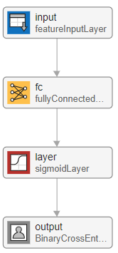
The first network is a simple neural network containing four layers.
Start with a feature input layer, which passes tabular data (credit panel data) to the network. In this example, there are four input features: YOB, HighRisk, MediumRisk, and LowRisk. Configure the input layer to normalize the data using z-score normalization. Normalizing the data is important for tasks where the scale and range of the input variables is very different.
Next, use a fully connected layer with a single output followed by a sigmoid layer. For the final layer, use a custom binary cross-entropy loss layer. This layer is attached to this example as a supporting file.
logisticLayers = [
    featureInputLayer(4,'Normalization','zscore')
    fullyConnectedLayer(1)
    sigmoidLayer];
This network is called a single-layer perceptron. You can visualize the network using Deep Network Designer or the analyzeNetwork function.
deepNetworkDesigner(logisticLayers)

You can easily show that the single-layer perceptron neural network is equivalent to logistic regression. Let be a 1-by-4 vector containing the features for observation . With input , the output of the fully connected layer is
.
The output of the fully connected layer provides the input for the sigmoid layer. The sigmoid layer then outputs
.
The output of the sigmoid layer is equivalent to the logistic regression model. The final layer of the neural network is a binary cross-entropy loss layer. Minimizing the binary cross-entropy loss is equivalent to maximizing the likelihood in a logistic regression model.
Multilayer Perceptron
The next network has a similar architecture to the logistic regression model, but has an additional fully connected layer with an output size of 100, followed by a ReLU nonlinear activation function. This type of network is called a multilayer perceptron due to the addition of another hidden layer and a nonlinear activation function. Whereas the single-layer perceptron can learn only linear functions, the multilayer perceptron can learn complex, nonlinear relationships between the input and output data.
mlpLayers = [
    featureInputLayer(4,'Normalization','zscore')
    fullyConnectedLayer(100)
    reluLayer
    fullyConnectedLayer(1)
    sigmoidLayer];

deepNetworkDesigner(mlpLayers)
Residual Network
For the final network, create a residual network (ResNet) [1] from multiple stacks of fully connected layers and ReLU activations. Originally developed for image classification, ResNets have proven successful across many domains. Because a ResNet has many more parameters than multilayer perceptrons or logistic networks, they take longer to train.
residualDLN = dlnetwork;
residualLayers = [
    featureInputLayer(4,'Normalization','zscore','Name','input')

    fullyConnectedLayer(16,'Name','fc1')
    batchNormalizationLayer('Name','bn1')
    reluLayer('Name','relu1')

    fullyConnectedLayer(32,'Name','resblock1-fc1')
    batchNormalizationLayer('Name','resblock1-bn1')
    reluLayer('Name','resblock1-relu1')

    fullyConnectedLayer(32,'Name','resblock1-fc2')
    additionLayer(2,'Name','resblock1-add')
    batchNormalizationLayer('Name','resblock1-bn2')
    reluLayer('Name','resblock1-relu2')

    fullyConnectedLayer(64,'Name','resblock2-fc1')
    batchNormalizationLayer('Name','resblock2-bn1')
    reluLayer('Name','resblock2-relu1')

    fullyConnectedLayer(64,'Name','resblock2-fc2')
    additionLayer(2,'Name','resblock2-add')
    batchNormalizationLayer('Name','resblock2-bn2')
    reluLayer('Name','resblock2-relu2')

    fullyConnectedLayer(1,'Name','fc2')
    sigmoidLayer('Name','sigmoid')];

residualDLN = addLayers(residualDLN,residualLayers);
residualDLN = addLayers(residualDLN,fullyConnectedLayer(32,'Name','resblock1-fc-shortcut'));
residualDLN = addLayers(residualDLN,fullyConnectedLayer(64,'Name','resblock2-fc-shortcut'));

residualDLN = connectLayers(residualDLN,'relu1','resblock1-fc-shortcut');
residualDLN = connectLayers(residualDLN,'resblock1-fc-shortcut','resblock1-add/in2');
residualDLN = connectLayers(residualDLN,'resblock1-relu2','resblock2-fc-shortcut');
residualDLN = connectLayers(residualDLN,'resblock2-fc-shortcut','resblock2-add/in2');

deepNetworkDesigner(residualDLN)
Network Depth
The depth of a network is an important concept in deep learning and is defined as the largest number of sequential convolutional or fully connected layers (represented by yellow blocks in the following diagram) on a path from the input layer to the output layer. The deeper a network is, the more complex features it can learn. In this example, the logistic network has a depth of 1, the multilayer perceptron has a depth of 2, and the residual network has a depth of 6.

Specify Training Options
Specify the training options.
Train using the Adam optimizer.
Set the initial learning rate to 0.001.
Set the mini-batch size to 512.
Turn on the training progress plot and turn off the command window output.
Shuffle the data at the beginning of each epoch.
Monitor the network accuracy during training by specifying validation data and using it to validate the network every 1000 iterations.
options = trainingOptions('adam', ...
    'InitialLearnRate',0.001, ...
    'MiniBatchSize',512, ...
    'Plots','training-progress', ...
    'Verbose',false, ...
    'Shuffle','every-epoch', ...
    'ValidationData',tblValidation, ...
    'ValidationFrequency',1000);
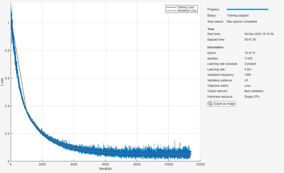
The loss landscape of the logistic regression network is convex, therefore, it does not need to train for as many epochs. For the logistic regression and multilayer perceptron models, train for 15 epochs. For the more complex residual network, train for 50 epochs.
logisticOptions = options;
logisticOptions.MaxEpochs = 15;

mlpOptions = options;
mlpOptions.MaxEpochs = 15;

residualOptions = options;
residualOptions.MaxEpochs = 50;
The three networks have different architectures, so they require different sets of training options to achieve optimal performance. You can perform optimization programmatically or interactively using Experiment Manager. For an example showing how to perform a hyperparameter sweep of the training options, see Compare Classification Network Architectures Using Experiment.
Train Network
Train the networks using the architectures defined, the training data, and the training options. By default, trainNetwork uses a GPU if one is available; otherwise, it uses a CPU. Training on a GPU requires Parallel Computing Toolbox™ and a supported GPU device. For information on supported devices, see GPU Computing Requirements (Parallel Computing Toolbox). You can also specify the execution environment by using the ExecutionEnvironment name-value argument of trainingOptions.
To avoid waiting for training, load pretrained networks by setting the doTrain flag to false. To train the networks using trainNetwork, set the doTrain flag to true.
Training times using a NVIDIA® GeForce® RTX 2080 Ti are:
Logistic network — Approximately 4 minutes
Multilayer perceptron — Approximately 5 minutes
Residual network — Approximately 35 minutes
doTrain = false;

if doTrain
    logisticNet = trainnet(tblTrain,logisticLayers,"binary-crossentropy",logisticOptions);
    mlpNet = trainnet(tblTrain,mlpLayers,"binary-crossentropy",mlpOptions);
    residualNet = trainnet(tblTrain,residualDLN,"binary-crossentropy",residualOptions);
else
    load logisticTrainedNetwork
    load mlpTrainedNetwork
    load residualTrainedNetwork
end


Test Network
Predict the default probability of the test data using the trained networks.
tblTest.logisticPred = predict(logisticNet,tblTest{:,1:4});
tblTest.mlpPred = predict(mlpNet,tblTest{:,1:4});
tblTest.residualPred = predict(residualNet,tblTest{:,1:4});
Default Rates by Year on Books
To assess the performance of the network, use the groupsummary function to group the true default rates and corresponding predictions by years on books (represented by the YOB variable) and calculate the mean value.
summaryYOB = groupsummary(tblTest,'YOB','mean',{'Default','logisticPred','mlpPred','residualPred'});
head(summaryYOB)
    YOB    GroupCount    mean_Default    mean_logisticPred    mean_mlpPred    mean_residualPred
    ___    __________    ____________    _________________    ____________    _________________

     1       19364         0.017352           0.017471          0.018056           0.017663
     2       18917         0.012158           0.014209          0.015486           0.014192
     3       18526         0.011875           0.011538          0.013154           0.011409
     4       18232         0.011683          0.0093902          0.011151           0.010311
     5       17925        0.0082008           0.007626         0.0089826          0.0093438
     6       17727        0.0066565          0.0062047         0.0062967          0.0073401
     7       12294        0.0030909          0.0050643         0.0042998          0.0047071
     8        6361        0.0017293          0.0041463         0.0029052          0.0025272
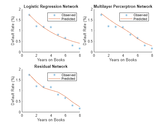
Plot the true average default rate against the average predictions by years on books.
networks = ["Logistic Regression Network","Multilayer Percerptron Network","Residual Network"];

figure
tiledlayout('flow','TileSpacing','compact')

for i = 1:3
    nexttile
    scatter(summaryYOB.YOB,summaryYOB.mean_Default*100,'*');
    hold on
    plot(summaryYOB.YOB,summaryYOB{:,i+3}*100);
    hold off
    title(networks(i))
    xlabel('Years on Books')
    ylabel('Default Rate (%)')
    legend('Observed','Predicted')
end


All three networks show a clear downward trend, with default rates going down as the number of years on books increases. Years three and four are an exception to the downward trend. Overall, the three models predict the default rates well, and even the simpler logistic regression model predicts the general trend. The residual network captures a more complex, nonlinear relationship compared to the logistic model, which can fit only a linear relationship.
Default Rates by Score Groups
Use the credit score group as a grouping variable to compute the observed and predicted default rate for each score group.
Decode ScoreGroup back into the categorical score groups.
ScoreGroup = onehotdecode(tblTest{:,2:4},{'HighRisk','MediumRisk','LowRisk'},2);
tblTest.ScoreGroup = ScoreGroup;
tblTest = removevars(tblTest,{'HighRisk','MediumRisk','LowRisk'});

riskGroups = categories(tblTest.ScoreGroup);
Use the groupsummary function to group the true default rate and the predictions by YOB and ScoreGroup, and return the mean for each group.
numYOB = height(summaryYOB);
numRiskGroups = height(riskGroups);

summaryYOBScore = groupsummary(tblTest,{'ScoreGroup','YOB'},'mean',{'Default','logisticPred','mlpPred','residualPred'});
head(summaryYOBScore)
ScoreGroup YOB GroupCount mean_Default mean_logisticPred mean_mlpPred mean_residualPred
__________ ___ __________ ____________ _________________ ____________ _________________
HighRisk 1 6424 0.029577 0.028404 0.031563 0.02973
HighRisk 2 6180 0.020065 0.02325 0.026649 0.023655
HighRisk 3 5949 0.019163 0.019013 0.022484 0.018724
HighRisk 4 5806 0.020668 0.015535 0.018957 0.017207
HighRisk 5 5634 0.01349 0.012686 0.01577 0.015374
HighRisk 6 5531 0.013379 0.010354 0.010799 0.01215
HighRisk 7 3862 0.0051787 0.0084466 0.0071398 0.0083738
HighRisk 8 2027 0.0034534 0.0068881 0.0047145 0.0040559
Plot the true average default rate against the predicted rate by years on books and risk group.
figure
t = tiledlayout('flow','TileSpacing','compact');
color = lines(3);

YOB = summaryYOBScore.YOB;
default = summaryYOBScore.mean_Default*100;
group = summaryYOBScore.ScoreGroup;

for i = 1:3
    pred = summaryYOBScore{:,i+4}*100;
    meanScore = reshape(pred,numYOB,numRiskGroups);

    nexttile
    hs = gscatter(YOB,default,group,color,'*',6,false);
    hold on
    colororder(color)
    plot(meanScore)
    hold off
    title(networks(i))
    xlabel('Years on Books')
    ylabel('Default Rate (%)')
    grid on
end

labels = ["True: " + riskGroups; "Pred: " + riskGroups];
lgd = legend(labels);
lgd.Layout.Tile = 4;


The plot shows that all score groups behave similarly as time progresses, with a general downward trend. Across the high risk group, year four does not follow the downward trend. In the medium risk group, years three and four appear flat. Finally, in the low risk group, year three shows an increase. These irregular trends are difficult to discern with the simpler logistic regression model.
For an example showing how to use the locally-interpretable model-agnostic explanations (LIME) and Shapley values interpretability techniques to understand the predictions of a residual network for credit default prediction, see Interpret and Stress-Test Deep Learning Networks for Probability of Default (Risk Management Toolbox).
References
[1] He, Kaiming, Xiangyu Zhang, Shaoqing Ren, and Jian Sun. "Deep residual learning for image recognition." In Proceedings of the IEEE conference on computer vision and pattern recognition, pp. 770-778. 2016.
See Also
trainnet | trainingOptions | dlnetwork | fullyConnectedLayer | Deep Network Designer | featureInputLayer
Topics
- Interpret and Stress-Test Deep Learning Networks for Probability of Default (Risk Management Toolbox)
- Hedge Options Using Reinforcement Learning Toolbox (Financial Toolbox)
- Create Simple Deep Learning Neural Network for Classification
- Train Convolutional Neural Network for Regression
- Deep Learning in MATLAB
- List of Deep Learning Layers