Improve Model Fit with Weights

This example shows how to fit a polynomial model to data using both the linear least-squares method and the weighted least-squares method for comparison.

Generate sample data from different normal distributions by using the randn function.

rng("default")  % For reproducibility

rnorm = [];
idx = [];

for k=1:20
    r = k*randn([20,1]) + (1/20)*(k^3);
    rnorm = [rnorm;r];
    idx = [idx;ones(20,1).*k];
end

The dependent variable rnorm contains sample data from 20 normal distributions. The independent variable idx contains integers indicating whether two elements in rnorm are sampled from the same normal distribution.

Fit a third-degree polynomial model to idx and rnorm. Return information about the coefficient estimates and the algorithm used to fit the model.

[p3fit,~,fitinfo] = fit(idx,rnorm,"poly3")

p3fit = 
     Linear model Poly3:
     p3fit(x) = p1*x^3 + p2*x^2 + p3*x + p4
     Coefficients (with 95% confidence bounds):
       p1 =     0.05156  (0.0438, 0.05932)
       p2 =    -0.03993  (-0.2875, 0.2076)
       p3 =      0.1418  (-2.124, 2.408)
       p4 =      0.0462  (-5.585, 5.678)

fitinfo = struct with fields:
        numobs: 400
      numparam: 4
     residuals: [400x1 double]
      Jacobian: [400x4 double]
      exitflag: 1
     algorithm: 'QR factorization and solve'
    iterations: 1

p3fit contains the estimates for the model coefficients with 95% confidence intervals. The default fitting method for fitting a polynomial model is linear least squares. fitinfo contains information about the fitting algorithm used to fit the coefficients to the data. The error in the data can be estimated by the residuals stored in fitinfo.

Plot the residuals using a stem plot.

stem(idx,fitinfo.residuals)
xlabel("idx")
ylabel("residuals")

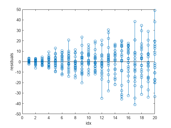
The plot of the residuals shows that their variance increases as the values in idx increase. The nonconstant variances across the different values of idx indicate that the weighted least-squares fitting method is more appropriate for calculating the model coefficients.

Create a vector of zeros for later storage of the weights.

W = zeros(length(rnorm),1);

The weights you supply transform the residual variances so that they are constant for different values of idx. Define the weight for each element in rnorm as the reciprocal of the residual variance for the corresponding value in idx. Then fit the model with the weights.

for k=1:20
    rnorm_idx = rnorm(idx==k);
    recipvar = 1/var(rnorm_idx);
    w = (idx==k).*recipvar;
    W = W+w;
end
[wp3fit,~,wfitinfo] = fit(idx,rnorm,"poly3","Weights",W)

wp3fit = 
     Linear model Poly3:
     wp3fit(x) = p1*x^3 + p2*x^2 + p3*x + p4
     Coefficients (with 95% confidence bounds):
       p1 =     0.04894  (0.04419, 0.0537)
       p2 =     0.03601  (-0.08744, 0.1595)
       p3 =     -0.4262  (-1.253, 0.4009)
       p4 =      0.9836  (-0.1959, 2.163)

wfitinfo = struct with fields:
        numobs: 400
      numparam: 4
     residuals: [400x1 double]
      Jacobian: [400x4 double]
      exitflag: 1
     algorithm: 'QR factorization and solve'
    iterations: 1

wp3fit and wfitinfo contain the results of the weighted least-squares fitting.

Display p3fit, wp3fit, and rnorm in the same plot.

plot(p3fit,idx,rnorm)
hold on
plot(wp3fit,"g")
xlabel("idx")
ylabel("rnorm")
legend(["rnorm","linear least-squares fit","weighted least-squares fit"])
hold off

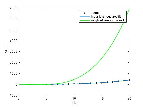
The plot shows wp3fit closely tracking p3fit.

You can determine whether wp3fit is a better fit than p3fit by plotting the residuals.

stem(idx,wfitinfo.residuals)
xlabel("idx")
ylabel("residuals")

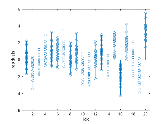
The output shows that the wp3fit residuals are smaller than the p3fit residuals. The variances of the wp3fit residuals are also more similar for different values of idx than the variances of the p3fit residuals.