Exponential Models

About Exponential Models

The toolbox provides a one-term and a two-term exponential model as given by

$$\begin{array}{l}y=a{e}^{bx}\\ y=a{e}^{bx}+c{e}^{dx}\end{array}$$

Exponentials are often used when the rate of change of a quantity is proportional to the initial amount of the quantity. If the coefficient associated with b and/or d is negative, y represents exponential decay. If the coefficient is positive, y represents exponential growth.

For example, a single radioactive decay mode of a nuclide is described by a one-term exponential. a is interpreted as the initial number of nuclei, b is the decay constant, x is time, and y is the number of remaining nuclei after a specific amount of time passes. If two decay modes exist, then you must use the two-term exponential model. For the second decay mode, you add another exponential term to the model.

Examples of exponential growth include contagious diseases for which a cure is unavailable, and biological populations whose growth is uninhibited by predation, environmental factors, and so on.

Fit Exponential Models Interactively

1. Open the Curve Fitter app by entering curveFitter at the MATLAB^® command line. Alternatively, on the Apps tab, in the Math, Statistics and Optimization group, click Curve Fitter.

2. In the Curve Fitter app, select curve data. On the Curve Fitter tab, in the Data section, click Select Data. In the Select Fitting Data dialog box, select X data and Y data, or just Y data against an index.

3. Click the arrow in the Fit Type section to open the gallery, and click Exponential in the Regression Models group.

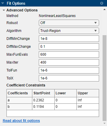
The Fit Options pane for the single-term Exponential fit is shown here.

You can specify the following options in the Fit Options pane:

• Choose one or two terms to fit exp1 or exp2. Look in the Results pane to see the model terms, values of the coefficients, and goodness-of-fit statistics.

• Optionally, in the Advanced Options section, specify coefficient starting values and constraint bounds appropriate for your data, or change algorithm settings. The coefficient starting values and constraints shown here are for the census data.

  The app calculates optimized start points for Exponential fits, based on the data set. You can override the start points and specify your own values in the Fit Options pane. For an example specifying starting values appropriate to the data, see Gaussian Fitting with an Exponential Background.

For more information on the settings, see Specify Fit Options and Optimized Starting Points.

Fit Exponential Models Using the fit Function

This example shows how to fit an exponential model to data using the fit function.

The exponential library model is an input argument to the fit and fittype functions. Specify the model type 'exp1' or 'exp2'.

Fit a Single-Term Exponential Model

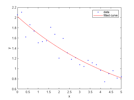
Generate data with an exponential trend and then fit the data using a single-term exponential. Plot the fit and data.

x = (0:0.2:5)';
y = 2*exp(-0.2*x) + 0.1*randn(size(x));
f = fit(x,y,'exp1')

f = 
     General model Exp1:
     f(x) = a*exp(b*x)
     Coefficients (with 95% confidence bounds):
       a =       2.021  (1.89, 2.151)
       b =     -0.1812  (-0.2104, -0.152)

plot(f,x,y)

Fit a Two-Term Exponential Model

f2 = fit(x,y,'exp2')

f2 = 
     General model Exp2:
     f2(x) = a*exp(b*x) + c*exp(d*x)
     Coefficients (with 95% confidence bounds):
       a =       384.8  (-4.78e+09, 4.78e+09)
       b =     -0.2572  (-2939, 2938)
       c =      -382.8  (-4.78e+09, 4.78e+09)
       d =     -0.2577  (-2957, 2957)

plot(f2,x,y)

Set Start Points

The toolbox calculates optimized start points for exponential fits based on the current data set. You can override the start points and specify your own values.

Find the order of the entries for coefficients in the first model ( f ) by using the coeffnames function.

coeffnames(f)

ans = 2x1 cell
    {'a'}
    {'b'}

If you specify start points, choose values appropriate to your data. Set arbitrary start points for coefficients a and b for example purposes.

f = fit(x,y,'exp1','StartPoint',[1,2])

f = 
     General model Exp1:
     f(x) = a*exp(b*x)
     Coefficients (with 95% confidence bounds):
       a =       2.021  (1.89, 2.151)
       b =     -0.1812  (-0.2104, -0.152)

plot(f,x,y)

Examine Exponential Fit Options

Examine the fit options if you want to modify fit options such as coefficient starting values and constraint bounds appropriate for your data, or change algorithm settings. For details on these options, see the table of properties for NonlinearLeastSquares on the fitoptions reference page.

fitoptions('exp1')

ans = 
  nlsqoptions with properties:

       StartPoint: []
            Lower: []
            Upper: []
        Algorithm: 'Trust-Region'
    DiffMinChange: 1.0000e-08
    DiffMaxChange: 0.1000
          Display: 'Notify'
      MaxFunEvals: 600
          MaxIter: 400
           TolFun: 1.0000e-06
             TolX: 1.0000e-06
           Robust: 'Off'
        Normalize: 'off'
          Exclude: []
          Weights: []
           Method: 'NonlinearLeastSquares'