xelim

Eliminate states from state-space models

Since R2023b

Syntax

rsys = xelim(sys,elim)

rsys = xelim(sys,elim,method)

Description

rsys = xelim(sys,elim) simplifies the state-space model sys by eliminating the states specified in the vector elim. The full state vector x is partitioned as x = [x₁;x₂] where x₁ is the reduced state vector and x₂ is eliminated.

This function is useful to eliminate states known to settle quickly (fast modes) or contribute little to the input/output map. When you don’t know which states to eliminate, use reducespec and the model-order reduction workflow.

rsys = xelim(sys,elim,method) also specifies the elimination method. Set method to either "MatchDC" or "Truncate".

Examples

Order Reduction by Matched-DC-Gain and Direct-Deletion Methods

Consider the following continuous fourth-order model.

$$h(s)=\frac{s^3+11s^2+36s+26}{s^4+14.6s^3+74.96s^2+153.7s+99.65}.$$

To reduce its order, first compute a balanced state-space realization with balreal.

h = tf([1 11 36 26],[1 14.6 74.96 153.7 99.65]);
[hb,g] = balreal(h);

Examine the Gramians.

g'

ans = 1×4

    0.1394    0.0095    0.0006    0.0000

The last three diagonal entries of the balanced Gramians are relatively small. Eliminate these three least-contributing states with xelim, using both matched DC gain and direct-deletion methods.

hmdc = xelim(hb,2:4,"MatchDC");
hdel = xelim(hb,2:4,"Truncate");

Both hmdc and hdel are first-order models. Compare their Bode responses against that of the original model.

bp = bodeplot(h,hmdc,'r--',hdel,'k-.');
bp.PhaseMatchingEnabled = 'on';
legend("Original","State elimination (match DC)",...
    "State elimination (truncate)");

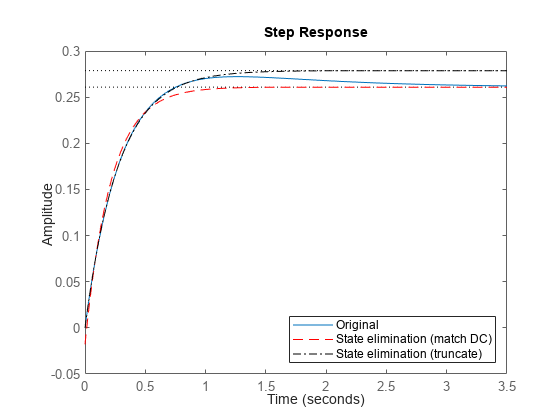
The reduced-order model hdel is clearly a better frequency-domain approximation of h. Now compare the step responses.

stepplot(h,hmdc,'r--',hdel,'k-.')
legend("Original","State elimination (match DC)",...
    "State elimination (truncate)",Location="southeast");

While hdel accurately reflects the transient behavior, only hmdc gives the true steady-state response.

For faster and more accurate results, use reducespec for model reduction workflows.

Find Matching Initial Condition for Reduced Model

Since R2024a

This example shows how to use findop to find the matching initial condition for a reduced model obtained with xelim.

Create a random state-space model.

rng(0)
sys = rss(10,1,2);

To reduce its order, first compute a balanced state-space realization with balreal.

[sysb,g] = balreal(sys);
g'

ans = 1×10

   13.2301    4.9468    1.0334    0.4597    0.0644    0.0287    0.0057    0.0007    0.0000    0.0000

Based on the small Gramians, you can eliminate last 6 states from balanced realization sysb.

rsys = xelim(sysb,5:10,"MatchDC");

With MatchDC option, the reduced model states may differ from ${\mathit{x}}_1$ because xelim scales and sometimes transforms the states $\mathit{x}$ to obtain the reduced model. Therefore, the initial conditions of the original model and reduced model may be different.

Compute the initial condition of the original and reduced models.

op = findop(sysb,u=[1 -1]);
opr = findop(rsys,u=[1 -1]);
op.x(1:4)

ans = 4×1

   18.9852
   -3.2735
    1.6693
    0.5918

opr.x

ans = 4×1

   18.9852
   -3.2735
    0.8347
    0.5918

The initial states for both models are different. Therefore, it is recommended to recompute the operating condition when reducing models. Using operating conditions of the original model with the reduced model may result in incorrect responses. For example, compare the initial response of the reduced model with the operating condition from the original model.

t = 0:0.01:5;
y = initial(sysb,op.x,t);
y1 = initial(rsys,op.x(1:4),t);
y2 = initial(rsys,opr.x,t);
plot(t,y,t,y1,'k:',t,y2,'r--')
legend("Original","Reduced (original IC)", "Reduced (recomputed IC)");

Input Arguments

sys — Dynamic system model

dynamic system model

Dynamic system model, specified as an ordinary or sparse LTI model.

The input model must have a valid state-space representation, such as tf, ss, sparss, mechss models. For generalized or uncertain state-space models (genss, uss), the function uses the current value of the model. For identified models (idss), the function uses the identified value.

elim — State elimination vector

vector

State elimination vector, specified as one of these.

• A vector containing index values of states you want to discard.

• A vector of logical values of the same size as the number of states, where the true (1) values specifies the states you want to discard.

method — State elimination method

"MatchDC" (default) | "Truncate"

State elimination method, specified as "MatchDC" or "Truncate". This argument specifies how the function eliminates the states with weak contribution.

• "MatchDC" — Enforce matching DC gains. To do so, the algorithm treats x₂ as infinitely fast and sets its derivative to zero. The resulting algebraic equation is used to express x₂ in terms of x₁ and eliminate it. For details, see Algorithms

• "Truncate" — Simply drop x₂, and use x₁ as reduced state.

The "Truncate" option tends to produce a better approximation in the frequency domain, but the DC gains are not guaranteed to match.

Output Arguments

rsys — Reduced-order model

state-space model

Reduced-order model, returned as a state-space model.

Algorithms

For a state-space model

$$\begin{array}{l}\dot{x}=Ax+Bu\\ y=Cx+Du\end{array}$$

the function partitions the state vector into x₁ (to keep) and x₂ (to eliminate).

$$\begin{array}{l}\left[\begin{array}{c}{\dot{x}}_1\\ {\dot{x}}_2\end{array}\right]=\left[\begin{array}{cc}{A}_{11}& A_{12}\\ A_{21}& A_{22}\end{array}\right]\left[\begin{array}{c}{x}_1\\ x_2\end{array}\right]+\left[\begin{array}{c}{B}_1\\ B_2\end{array}\right]u\\ y=\left[\begin{array}{cc}{C}_1& C_2\end{array}\right]x+Du\end{array}$$

"MatchDC" Method

For continuous-time models, this method sets the derivative of x₂ to zero and solves the resulting equation for x₁. The reduced-order model is given by

$$\begin{array}{l}{\dot{x}}_1=\left[A_{11}-A_{12}{A}_{22}{}^{-1}{A}_{21}\right]x_1+\left[B_1-A_{12}{A}_{22}{}^{-1}{B}_2\right]u\\ y=\left[C_1-C_2{A}_{22}{}^{-1}{A}_{21}\right]x+\left[D-C_2{A}_{22}{}^{-1}{B}_2\right]u\end{array}$$

Similarly, for discrete-time models, the algorithm sets $$x_2[n+1]=x_2[n]$$ to recompute the matrices.

These equations of the algorithm describe only the general idea. The function performs additional scaling and eliminates only a portion of x₂ when A₂₂ or A₂₂ – E₂₂ is nearly singular. This alters x₁ and the original initial condition x₁(0) is not valid. You can use the findop function to compute matching initial conditions for the reduced model. For an example, see Find Matching Initial Condition for Reduced Model.

"Truncate" Method

For this method, the algorithm simply drops x₂, and uses x₁ as reduced state. The reduced-order model is given by

$$\begin{array}{l}{\dot{x}}_1=A_{11}{x}_1+B_{1}u\\ y=C_1{x}_1\end{array}$$

xelim returns a scaled version of this realization.

Version History

Introduced in R2023b