initial
System response to initial states of state-space model
Syntax
Description
For state-space and sparse state-space models, initial
computes the unforced system response y to initial states
xinit.
Continuous time:
Discrete time:
For linear time-varying or linear parameter-varying state-space models,
initial computes the response with initial state
xinit, initial parameter
pinit (LPV models), and input held to the offset
value (u(t) =
u0(t) or u(t) =
u0(t,p). This corresponds to the initial condition response of the local linear
dynamics.
initial(
plots the initial response of sys,xinit,___)sys. This syntax is equivalent to
initialplot(sys,__). When you need additional plot customization
options, use initialplot instead.
Examples
Initial Conditions Response Plot
For this example, generate a random state-space model with 5 states and create the plot for the system response to the initial states.
rng("default")
sys = rss(5);
x0 = [1,2,3,4,5];
initial(sys,x0)
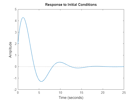
Response of State-Space Model to Initial Condition
Plot the response of the following state-space model:
Take the following initial condition:
a = [-0.5572, -0.7814; 0.7814, 0];
c = [1.9691  6.4493];
x0 = [1 ; 0];

sys = ss(a,[],c,[]);
initial(sys,x0)
Initial Condition Response Plot of MIMO System
Consider the following two-input, two-output dynamic system.
Convert the sys to state-space form since initial condition response plots are supported only for state-space models.
sys = ss([0, tf([3 0],[1 1 10]) ; tf([1 1],[1 5]), tf(2,[1 6])]);
size(sys)
State-space model with 2 outputs, 2 inputs, and 4 states.
The resultant state-space model has four states. Hence, provide an initial condition vector with four elements.
x0 = [0.3,0.25,1,4];
Create the initial condition response plot.
initial(sys,x0);

The resultant plot contains two subplots - one for each output in sys.
Initial Conditions Response Plot at Specified Time
For this example, examine the initial condition response of the following zero-pole-gain model and limit the plot to tFinal = 15 s.
First, convert the zpk model to an ss model since initial only supports state-space models.
sys = ss(zpk(-1,[-0.2+3j,-0.2-3j],1)*tf([1 1],[1 0.05]));
tFinal = 15;
x0 = [4,2,3];
Now, create the initial conditions response plot.
initial(sys,x0,tFinal);

Initial Condition Responses of Multiple Systems
For this example, plot the initial condition responses of three dynamic systems.
First, create the three models and provide the initial conditions. All the models should have the same number of states.
rng('default');
sys1 = rss(4);
sys2 = rss(4);
sys3 = rss(4);
x0 = [1,1,1,1];
Plot the initial condition responses of the three models using time vector t that spans 5 seconds.
t = 0:0.1:5;
initial(sys1,'r--',sys2,'b',sys3,'g-.',x0,t)

Initial Condition Response Data of State-Space Model
Extract the initial condition response data of the following state-space model with two states:
Use the following initial conditions:
a = [-0.5572, -0.7814; 0.7814, 0];
c = [1.9691  6.4493];
x0 = [1 ; 0];
sys = ss(a,[],c,[]);
[y,tOut,x] = initial(sys,x0);
The array y has as many rows as time samples (length of tOut) and as many columns as outputs. Similarly, x has rows equal to the number of time samples (length of tOut) and as many columns as states.
Initial Condition Response Data with Specified Time
For this example, extract the initial condition response data of a state-space model with 6 states, 3 outputs and 2 inputs.
First, create the model and provide the initial conditions.
rng('default');
sys = rss(6,3,2);
x0 = [0.1,0.3,0.05,0.4,0.75,1];
Extract the initial condition responses of the model using time vector t that spans 15 seconds.
t = 0:0.1:15;
[y,tOut,x] = initial(sys,x0,t);
The array y has as many rows as time samples (length of tOut) and as many columns as outputs. Similarly, x has rows equal to the number of time samples (length of tOut) and as many columns as states.
Initial Response of Linear-Parameter Varying State-Space Model
For this example, throttleLPV.m that defines the dynamics of a nonlinear engine throttle which behaves linearly in the 15 degrees to 90 degrees opening range.
Use lpvss to create the model. This model is parameterized by the throttle angle, which is the first state of the model.
c0 = 50;
k0 = 120;
K0 = 1e4;
b0 = 4e4;
yf = 15*K0/(k0+K0);
Ts = 0;
sys = lpvss("x1",@(t,p) throttleLPV(p,c0,k0,b0,K0),Ts,0,15);
You can compute the initial response for this model along a trajectory .
Compute the response when you start at the lower end of linear range with a small angular velocity.
pFcn = @(t,x,u)x(1);
x0 = [15;10];
p0 = x0(1);
t = linspace(0,0.6,500);
initial(sys,{x0,p0},t,pFcn)
Compute the response when you start at the lower end of linear range with enough angular velocity to hit the upper end of this range.
x0 = [15;5e3];
p0 = x0(1);
t = linspace(0,1,1000);
initial(sys,{x0,p0},t,pFcn)
View the data function.
type throttleLPV.mfunction [A,B,C,D,E,dx0,x0,u0,y0,Delays] = throttleLPV(x1,c,k,b,K) % LPV representation of engine throttle dynamics. % Ref: https://www.mathworks.com/help/sldo/ug/estimate-model-parameter-values-gui.html % x1: scheduling parameter (throttle angle; first state of the model) % c,k,b,K: physical parameters A = [0 1; -k -c]; B = [0; b]; C = [1 0]; D = 0; E = []; Delays = []; x0 = []; u0 = []; y0 = []; % Nonlinear displacement value NLx = max(90,x1(1))-90+min(x1(1),15)-15; % Capture the nonlinear contribution as a state-derivative offset dx0 = [0;-K*NLx];
Input Arguments
Output Arguments
Version History
Introduced before R2006aSee Also
initialplot | impulse | lsim | Linear System Analyzer | step
You can also select a web site from the following list:
Americas
- América Latina (Español)
- Canada (English)
- United States (English)
Europe
- Belgium (English)
- Denmark (English)
- Deutschland (Deutsch)
- España (Español)
- Finland (English)
- France (Français)
- Ireland (English)
- Italia (Italiano)
- Luxembourg (English)
- Netherlands (English)
- Norway (English)
- Österreich (Deutsch)
- Portugal (English)
- Sweden (English)
- Switzerland
- United Kingdom (English)