UWB Channel Models
This example shows how to implement and equalize UWB channel models for a variety of propagation environments. The implementation is based on recommendations from the channel modeling subgroup of IEEE® 802.15.4a™ [ 1 ]. You can reuse these UWB channel models for the IEEE 802.15.4ab/z amendments [ 2 ], which enhance the HRP PHY introduced by IEEE 802.15.4a.
Background
The recommended UWB channel models comprise the following parts:
Application of distance- and frequency-dependent path loss
A modified Saleh-Valenzuela model [ 3 ], which contains multipath components that are grouped in distinct clusters
Determination of path amplitudes with distinct Nakagami distributions (small-scale fading)
Environment-specific parameterization of the above steps
Channel Parameterization
Environment
The IEEE 802.15.4a channel modeling subgroup recommends multiple UWB models for the 2 to 10 GHz range, which cover a wide range of environments:
Residential (indoor)
Indoor office
Outdoor (suburban-like)
Open outdoor (agricultural)
Industrial (indoor)
The subgroup recommends a LOS and a non-LOS model for each environment type, except for open outdoor, depending on the presence of a line-of-sight (LOS) component. Therefore, this example implements a total of nine combinations (type x LOS) for the 2 to 10 GHz range.
environmentType ="Residential"; LOS =
true;
Frequency-Dependent Path Loss
Different frequencies of the UWB channel bandwidth experience dissimilar frequency-dependent path loss: .
The environment and LOS configuration determine the frequency exponent κ. The channel specification in the IEEE 802.15.4a/z amendments determines the center frequency and channel bandwidth.
channelSpec =[0 499.2e6 499.2e6]; channelNum = channelSpec(1); Fc = channelSpec(2); bw = channelSpec(3); fprintf('Channel #%d: Center frequency = %.1f MHz, Bandwidth = %.1f MHz.\n', channelNum, Fc/1e6, bw/1e6);
Channel #0: Center frequency = 499.2 MHz, Bandwidth = 499.2 MHz.
Distance-Dependent Path Loss
The UWB channel model also exhibits distance-dependent path loss, as per the classic log distance propagation model:
d =10; % distance between transmitter and receiver, in meters
The environment and LOS configuration determine the path loss exponent n, the reference path loss PL0, and the deviation of shadowing (S).
Clusterized Multipath Fading
Each UWB channel has a number of clusters; a cluster is a collection of nearby multi-path components. For most environment types, the number of clusters is a random number that is specific to a channel instance and follows a Poisson distribution. The interrarival times between successive clusters and between successive multipath components of the same cluster are both exponentially distributed. The average path power within a cluster decays exponentially.
However, the "Indoor office" NLOS and "Industrial" NLOS environments always specify a single cluster that has regular (continuous) tap spacings. The average path power initially increases with path delay, up to a certain maximum, and then decays.
The environment and LOS configuration determine the statistics of the Poisson and exponential distributions, as well as parameters affecting the average power of each path. The info method of uwbChannel describes the realized cluster and path setup in detail.
Small-Scale Fading (Nakagami)
Each multipath component exhibits Nakagami small-scale fading. The environment and LOS configuration, as well as the path delay, determine the Nakagami parameters.
The timescale of small-scale fading is controlled by the SampleDensity and MaxDopplerShift properties of the uwbChannel object. Specifically, the rate of channel realizations is Fcg = 2 * SampleDensity * MaxDopplerShift. In other words, the coherence time is 1/Fcg = 1/(2 * SampleDensity * MaxDopplerShift) seconds, or cfgHPRF.SampleRate/(2 * SampleDensity * MaxDopplerShift) samples of the input signal.
sampleDensity =10000; maxDopplerShift =
5; % in Hz
Transmitted Signal
Any signal can be passed to the UWB channel, but IEEE 802.15.4a/z/ab UWB waveforms are of the most relevant type. The HRP UWB IEEE 802.15.4a/z Waveform Generation example illustrates how to create such waveforms; the following section creates an HPRF UWB waveform:
% Create an HPRF IEEE 802.15.4z signal:
rng(17)
msg = randi([0 1], 1000, 1);
cfgHPRF = lrwpanHRPConfig(Mode='HPRF',PSDULength=length(msg)/8);
waveHPRF = lrwpanWaveformGenerator(msg,cfgHPRF);
Filtering and Visualization
You can use the above channel-configuration parameters to create the respective UWB channel, then filter any UWB waveform with it, and visualize the channel impulse response (CIR).
uwbChan = uwbChannel(environmentType, LOS, ChannelNumber=channelNum, Distance=d, ...
  SampleRate=cfgHPRF.SampleRate, SampleDensity=sampleDensity, MaxDopplerShift=maxDopplerShift, ...
  Visualization="Impulse response");
rcvSig = uwbChan(waveHPRF); % filter UWB waveform
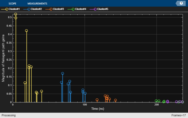
s = info(uwbChan) % display info about the UWB channels = struct with fields:
EnvironmentParameterization: [1×1 struct]
CenterFrequency: 499200000
Bandwidth: 499200000
NumClusters: 5
ClusterArrivalTimes: [4.1103 67.8509 117.3937 199.6441 215.4132]
ClusterEnergies: [0.7473 0.0827 0.0079 1.5887e-04 6.9327e-05]
PathArrivalTimes: {[0 0.1663 12.9858 15.0197 18.5857 18.7689 21.6895 28.7055 29.6166 35.9837] [0 1.5615 9.2612 11.4917 12.5556 29.7187 29.7918 32.9943] [0 11.3300 13.7646 13.8394 14.1783 17.1480 25.6085] [1×6 double] [1×5 double]}
AbsolutePathArrivalTimes: {1×5 cell}
PathAveragePowers: {1×5 cell}
PathPhases: {[5.1362 2.3422 5.6201 1.3803 0.8222 1.5764 0.7143 0.5807 3.7371 4.3481] [2.7708 0.1260 5.0393 0.6088 1.5105 5.1944 2.9207 0.4019] [1.8693 1.6542 5.0820 6.2699 1.3549 4.4068 6.2540] [1×6 double] [1×5 double]}
NakagamiMFactors: {[1.3287 2.2944 2.3048 1.5491 1.8249 1.7147 2.7704 2.4127 1.0488 1.3357] [3.0777 1.9799 2.3824 2.4898 2.4369 4.0513 2.6362 2.4376] [1.6535 2.2602 2.1196 1.3875 0.9916 2.2804 1.9402] [1×6 double] [1×5 double]}
PathGainRate: 100000
FrequencyFilterDelay: 25
ChannelFilterDelay: 0
ChannelFilterCoefficients: [36×480 double]
Environment Comparison
You can visualize the channel gains for different environments, to illustrate key differences in their power delay profiles.
Alternate PDP
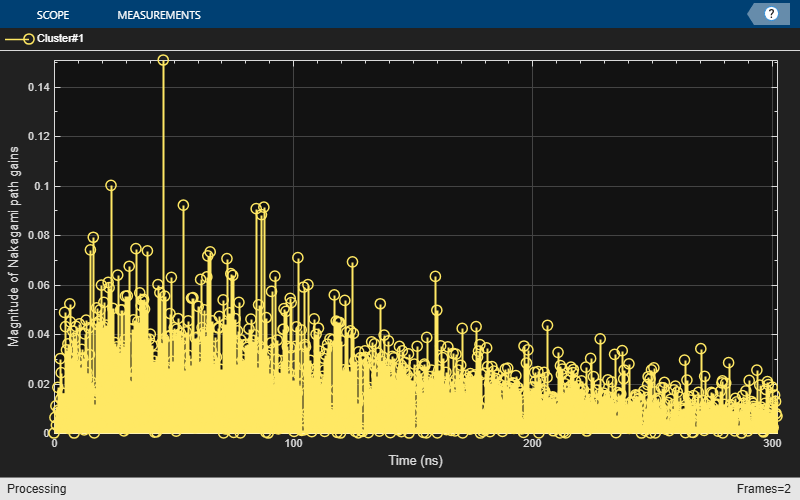
First, the industrial NLOS environment differs in that it consists of a single cluster with regular tap spacings. The PDP shape first increases and then decays.
NLOS = false;
industrialUWBChannel = uwbChannel('Industrial', NLOS, ...
    Distance = 10, ...
    ChannelNumber = 0, ...
    MinRelativePathPower = 5, ...
    SampleRate = 499.2*10*1e6, ...
    SampleDensity = 1e5, ...
    MaxDopplerShift = 5, ...
    Visualization = 'Impulse response');
% waveTx = lrwpanWaveformGenerator(psdu, cfgHPRF);  % start with a clean signal
% waveRx = industrialUWBChannel(waveTx);            % pass Tx signal through the wireless channel
industrialUWBChannel(zeros(0, 1));                  % visualize channel realization, without signal filtering
Outdoor environments
The outdoor UWB environment differs in that its average number of clusters is typically substantially higher.
outdoorUWBChannel = uwbChannel('Outdoor', NLOS, Visualization = 'Impulse response');
outdoorUWBChannel(zeros(0, 1));                     % only obtain channel realization

Equalization
You can mitigate the effects of the UWB multipath channel via an equalizer. The following section uses an LMS equalizer to correct the received UWB signal. You can then calculate BER to quantify the effectiveness of multipath mitigation.
Transmitted Signal
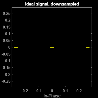
This example transmits an HPRF 15.4z waveform over a Residential UWB channel. HRP UWB frames follow a ternary ([-1 0 1]) constellation, which the scatterplot function can illustrate.
msg = randi([0 1], 1000, 1);
cfgHPRF = lrwpanHRPConfig(Mode='HPRF',PSDULength=length(msg)/8);
waveHPRF = lrwpanWaveformGenerator(msg,cfgHPRF);
scatterplot(waveHPRF(cfgHPRF.SamplesPerPulse:cfgHPRF.SamplesPerPulse:end));
title('Ideal signal, downsampled');
The LMS equalizer needs a known preamble that is not oversampled.The 802.15.4a/z/ab UWB waveforms contain a known code sequence that is repeated a total of PreambleDuration times. To obtain the pre-oversampling preamble, you can use the lrwpanHRPFieldIndices helper function to obtain the end and start of the SYNC (preamble) field, as well as property values of the lrwpanHRPConfig object to perform the right indexing operations.
ind = lrwpanHRPFieldIndices(cfgHPRF);
preambleSampPerRepet = (diff(ind.SYNC)+1)/cfgHPRF.PreambleDuration;  % number of preamble samples per repetition
repetAllowed = floor((length(waveHPRF)/cfgHPRF.SamplesPerPulse)/preambleSampPerRepet); % equalizer needs trainingLength <= length(input)/OSR
numRepet = min(cfgHPRF.PreambleDuration, repetAllowed);
preambleDownSampled = waveHPRF(ind.SYNC(1): cfgHPRF.SamplesPerPulse: numRepet*preambleSampPerRepet);
UWB Multipath Channel
Next, you can enable and visualize the multi-path effects specified in [ 1 ], by using the uwbChannel object and the scatterplot function, respectively.
LOS = true;
chanUWB = uwbChannel('Residential', LOS, SampleRate=cfgHPRF.SampleRate, ...
                      RandomStream='mt19937ar with seed', Seed=209);
mpathHPRF = chanUWB(waveHPRF);   % transmission
s = info(chanUWB);
fprintf('Number of clusters = %d\n', s.NumClusters);
Number of clusters = 5
scatterplot(mpathHPRF);
title('Multipath, oversampled');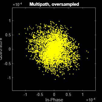
LMS Equalization
As a first step towards equalization, you need to control the gain of the received 15.4z signal, so that its power is at the same levels with the Constellation property of the equalizer.
constelScale = max(abs(preambleDownSampled));
mpathHPRF = mpathHPRF * constelScale * 1/max(abs(mpathHPRF));
Next, you can use comm.LinearEqualizer to equalize UWB signals that have experienced multipath fading. Towards this end, the equalizer needs to be set up for a specific channel construction (by a proper NumTaps, ReferenceTap, StepSize specification); the equalizer does not automatically adjust its operation to different channel realizations (Number of clusters, channel impulse response). In the following code, you can see an example that sets up an LMS equalizer for the 5-cluster residential UWB channel constructed above.
lmsEq = comm.LinearEqualizer(Algorithm="LMS", Constellation=[-1 0 1]*constelScale, InputSamplesPerSymbol=cfgHPRF.SamplesPerPulse, ...
  NumTaps=220, ReferenceTap=80, StepSize=0.2);
eqLatency = info(lmsEq).Latency; % in symbols

[eqHPRF, errLMS, w] = lmsEq([mpathHPRF; zeros(eqLatency*cfgHPRF.SamplesPerPulse, 1)], preambleDownSampled);
scatterplot(eqHPRF(numRepet*preambleSampPerRepet+4:end));
title('Equalized, downsampled');
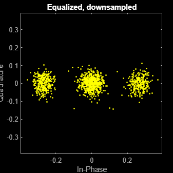
You can observe the successful equalization as the constellation now resembles the original ternary constellation ([-1 0 1]) that was transmitted.
Finally, you can decode the equalized signal using the helper function lrwpanWaveformDecoder. This function expects the meaninfgful signal content at the start of its input, without a delay, i.e., it does not perform preamble detection.
cfgHPRF.SamplesPerPulse = 1; % equalizer decimates
rcvPSDU = lrwpanWaveformDecoder([eqHPRF(1+eqLatency+1:end); 0], cfgHPRF);
Now that the equalized signal has been decoded, you can compare it to its transmitted version by computing the bit error rate.
[~, ber] = biterr(msg, rcvPSDU);
fprintf('BER=%f\n', ber);
BER=0.000000
Further Exploration
To further explore this example, you can modify the environment type and the LOS setting. You can give different values for the channel number, the distance between the two link endpoints, and the Doppler shift.
Moreover, you can set up the equalizer for different channel realizations (different environment, number of clusters, cluster and path delays).
References
1. A. F. Molisch et al., “IEEE 802.15.4a Channel Model-Final Report,” Tech. Rep., Document IEEE 802.1504-0062-02-004a, 2005.
2. "IEEE Standard for Low-Rate Wireless Networks--Amendment 1: Enhanced Ultra Wideband (UWB) Physical Layers (PHYs) and Associated Ranging Techniques," in IEEE Std 802.15.4z-2020 (Amendment to IEEE Std 802.15.4-2020), pp.1–174, 25 August 2020, DOI: 10.1109/IEEESTD.2020.9179124.
3. A. Saleh and R. A. Valenzuela, “A statistical model for indoor multipath propagation,” IEEE J. Selected Areas Comm., Vol. 5, pp. 138–137, February 1987.