raypl

Path loss and phase change for RF propagation ray

Since R2020a

Syntax

[pl,phase] = raypl(ray)

[pl,phase] = raypl(ray,Name,Value)

Description

[pl,phase] = raypl(ray) returns the path loss pl in dB and phase shift phase in radians for the RF propagation ray ray. The function calculates the path loss and phase shift using free space loss and reflection loss derived from the propagation path, reflection materials, and antenna polarizations.

By default, raypl assumes the antennas are unpolarized. You can polarize the antennas by specifying the TransmitterPolarization and ReceiverPolarization name-value arguments.

For more information about the path loss computations, see Path Loss Computation.

[pl,phase] = raypl(ray,Name,Value) specifies options using name-value arguments. For example, "ReflectionMaterials","brick" specifies the reflection material as brick.

Examples

Reevaluate Path Loss Changing Reflection Materials and Frequency

Change the reflection materials and frequency for a ray, and then reevaluate the path loss and phase shift.

Launch Site Viewer with buildings in Hong Kong. For more information about the OpenStreetMap® file, see [1].

viewer = siteviewer("Buildings","hongkong.osm");

Create transmitter and receiver sites.

tx = txsite("Latitude",22.2789,"Longitude",114.1625, ...
    "AntennaHeight",10,"TransmitterPower",5, ...
    "TransmitterFrequency",28e9);
rx = rxsite("Latitude",22.2799,"Longitude",114.1617, ...
    "AntennaHeight",1);

Create a ray tracing propagation model, which MATLAB® represents using a RayTracing object. Configure the model to use the image method and to find paths with up to 2 surface reflections. Then, perform the ray tracing analysis.

pm = propagationModel("raytracing", ...
    "Method","image", ...
    "MaxNumReflections",2);
rays = raytrace(tx,rx,pm);

Find the first ray with two path reflections. Then, display the properties of the ray object.

idx = find([rays{1}.NumInteractions] == 2,1);
ray = rays{1}(idx)

ray = 
  Ray with properties:

      PathSpecification: 'Locations'
       CoordinateSystem: 'Geographic'
    TransmitterLocation: [3×1 double]
       ReceiverLocation: [3×1 double]
            LineOfSight: 0
           Interactions: [1×2 struct]
              Frequency: 2.8000e+10
         PathLossSource: 'Custom'
               PathLoss: 121.8188
             PhaseShift: 4.5601

   Read-only properties:
       PropagationDelay: 8.3060e-07
    PropagationDistance: 249.0068
       AngleOfDeparture: [2×1 double]
         AngleOfArrival: [2×1 double]
        NumInteractions: 2

Display the ray in Site Viewer.

plot(ray)

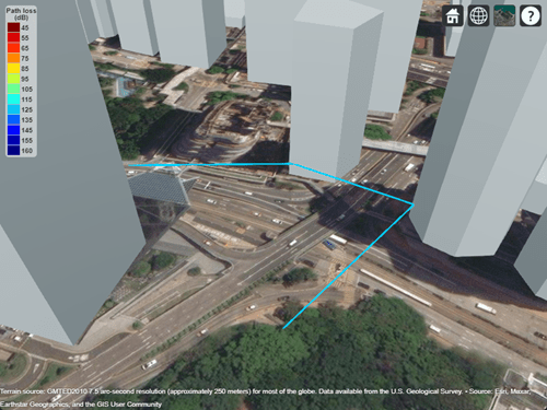
By default, the model uses concrete for the terrain material and uses building materials derived from the OpenStreetMap file. When the OpenStreeMap file does not specify materials, the model uses concrete. In this case, the ray encounters concrete as the material. You can find the interaction materials by querying the Interactions property of the ray object.

ray.Interactions.MaterialName

ans = 
"concrete"

ans = 
"concrete"

You can calculate the path loss for different materials by using the raypl function. For this example, use metal for the first reflection and glass for the second reflection.

[ray.PathLoss,ray.PhaseShift] = raypl(ray,"ReflectionMaterials",["metal" "glass"]);
ray

ray = 
  Ray with properties:

      PathSpecification: 'Locations'
       CoordinateSystem: 'Geographic'
    TransmitterLocation: [3×1 double]
       ReceiverLocation: [3×1 double]
            LineOfSight: 0
           Interactions: [1×2 struct]
              Frequency: 2.8000e+10
         PathLossSource: 'Custom'
               PathLoss: 114.9493
             PhaseShift: 4.5601

   Read-only properties:
       PropagationDelay: 8.3060e-07
    PropagationDistance: 249.0068
       AngleOfDeparture: [2×1 double]
         AngleOfArrival: [2×1 double]
        NumInteractions: 2

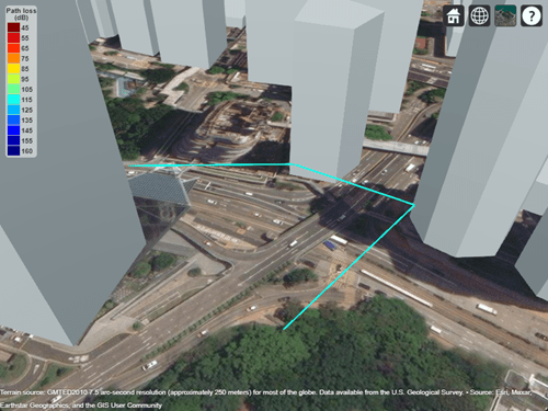
Display the recalculated ray. The slight change in color indicates the change in path loss.

plot(ray)

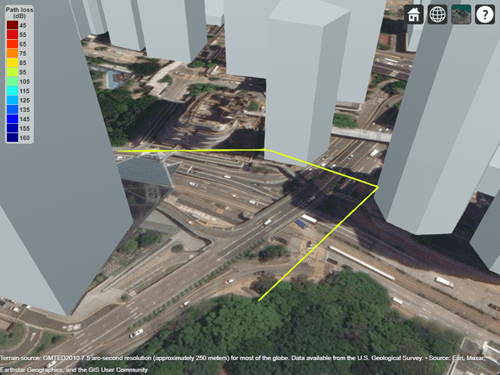
Change the frequency of the ray. Then, recalculate the path loss and phase shift. Display the ray again and observe the color change.

ray.Frequency = 2e9;
[ray.PathLoss,ray.PhaseShift] = raypl(ray,"ReflectionMaterials",["metal","glass"]);
plot(ray)

Appendix

[1] The OpenStreetMap file is downloaded from https://www.openstreetmap.org, which provides access to crowd-sourced map data all over the world. The data is licensed under the Open Data Commons Open Database License (ODbL), https://opendatacommons.org/licenses/odbl/.

Input Arguments

ray — RF propagation ray

comm.Ray object

RF propagation ray, specified as one comm.Ray object. The PathSpecification property of the object must be "Locations". All interactions in the Interactions property of the ray must be of type "Reflection".

Data Types: comm.Ray

Name-Value Arguments

Specify optional pairs of arguments as Name1=Value1,...,NameN=ValueN, where Name is the argument name and Value is the corresponding value. Name-value arguments must appear after other arguments, but the order of the pairs does not matter.

Before R2021a, use commas to separate each name and value, and enclose Name in quotes.

Example: raypl(ray,"TransmitterPolarization","H","ReceiverPolarization","H"), specifies the horizontal polarizations for the transmit and receive antennas for ray.

ReflectionMaterials — Reflection materials

"concrete" (default) | string scalar | 1-by-NR string vector | character vector | 1-by-NR cell array of character vectors | 2-by-1 numeric vector | 2-by-NR numeric matrix

Reflection materials for a non-line-of-sight (NLOS) ray, specified as a string scalar, a 1-by-NR string vector, a character vector, a 1-by-NR cell array of character vectors, a 2-by-1 numeric vector, or a 2-by-NR numeric matrix. NR is the number of reflections stored in ray.

When you specify one reflection material, the reflection material applies to all the reflections. When you specify multiple reflection materials, each material applies to the associated reflection point in ray.

• To use predefined reflection materials, specify ReflectionMaterials as a string scalar, a character vector, a string vector, or a cell array of character vectors. Specify each reflection material as one of these options: "concrete", "brick", "wood", "glass", "plasterboard", "ceiling-board", "chipboard", "floorboard", "metal", "water", "vegetation", "loam", or "perfect-reflector".

• To use custom reflection materials, specify a 2-by-1 numeric vector or a 2-by-NR numeric matrix. Each column is of the form [rp; cv], where rp is the relative permittivity and cv is the conductivity.

For more information, see ITU Permittivity and Conductivity Values for Common Materials.

Example: "ReflectionMaterials",["concrete","water"], specifies that a ray with two reflections uses the electrical characteristics of concrete at the first reflection point and water at the second reflection point.

Data Types: string | char | double

TransmitterPolarization — Transmit antenna polarization type

"none" (default) | "V" | "H" | "LHCP" | "RHCP" | normalized 2-by-1 Jones vector

Transmit antenna polarization type, specified as one of these values:

• "none" — Unpolarized

• "V" — Linearly polarized in the vertical (θ) direction

• "H" — Linearly polarized in the horizontal (φ) direction

• "LHCP" — Left-hand circular polarized

• "RHCP" — Right-hand circular polarized

• A normalized 2-by-1 Jones vector (also called a polarization matrix) of the form [H;V], where H is the horizontal component and V is the vertical component.

For more information about polarization types and Jones vectors, see Jones Vector Notation.

Example: "TransmitterPolarization","RHCP" specifies right-hand circular polarization for the transmit antenna.

Data Types: double | char | string

ReceiverPolarization — Receive antenna polarization type

"none" (default) | "V" | "H" | "LHCP" | "RHCP" | normalized 2-by-1 Jones vector

Receive antenna polarization type, specified as one of these values:

• "none" — Unpolarized

• "V" — Linearly polarized in the vertical (θ) direction

• "H" — Linearly polarized in the horizontal (φ) direction

• "LHCP" — Left-hand circular polarized

• "RHCP" — Right-hand circular polarized

• A normalized 2-by-1 Jones vector (also called a polarization matrix) of the form [H;V], where H is the horizontal component and V is the vertical component.

For more information about polarization types and Jones vectors, see Jones Vector Notation.

Example: "ReceiverPolarization",[1;0] specifies horizontal polarization for the receive antenna by using Jones vector notation.

Data Types: double | char | string

TransmitterAxes — Orientation of transmit antenna axes

3-by-3 identity matrix (default) | 3-by-3 unitary matrix

Orientation of the transmit antenna axes, specified as a 3-by-3 unitary matrix indicating the rotation from the transmitter local coordinate system (LCS) into the global coordinate system (GCS). When the CoordinateSystem property of the comm.Ray is set to "Geographic", the GCS orientation is the local East-North-Up (ENU) coordinate system at transmitter. For more information, see Coordinate System Orientation.

Example: "TransmitterAxes",eye(3), specifies that the local coordinate system for the transmitter axes is aligned with the global coordinate system. This is the default orientation.

Data Types: double

ReceiverAxes — Orientation of receive antenna axes

3-by-3 identity matrix (default) | 3-by-3 unitary matrix

Orientation of the receive antenna axes, specified as a 3-by-3 unitary matrix indicating the rotation from the receiver local coordinate system (LCS) into the global coordinate system (GCS). The GCS orientation is the local East-North-Up (ENU) coordinate system at receiver when the CoordinateSystem property of the comm.Ray is set to "Geographic". For more information, see Coordinate System Orientation.

Example: "ReceiverAxes",[0 -1 0; 1 0 0; 0 0 1], specifies a 90° rotation around the z-axis of the local receiver coordinate system with respect to the global coordinate system.

Data Types: double

Output Arguments

pl — Path loss

nonnegative scalar

Path loss in dB, returned as a nonnegative scalar.

Data Types: double

phase — Phase shift

scalar

Phase shift in radians, returned as a scalar in the range [–π, π] radians. The argument uses the e^-iωt time convention.

Data Types: double

More About

ITU Permittivity and Conductivity Values for Common Materials

ITU-R P.2040-1 [2] and ITU-R P.527-5 [3] present methods, equations, and values used to calculate real relative permittivity, conductivity, and complex relative permittivity for the common materials.

• For information about the values computed for building materials specified in ITU-R P.2040-1, see buildingMaterialPermittivity.

• For information about the values computed for terrain materials specified in ITU-R P.527-5, see earthSurfacePermittivity.

Coordinate System Orientation

This image shows the orientation of the electromagnetic fields in the global coordinate system (GCS) and the local coordinate systems of the transmitter and receiver.

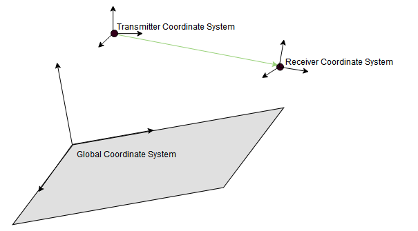
When the CoordinateSystem property of the comm.Ray is set to "Geographic", the GCS orientation is the local East-North-Up (ENU) coordinate system at observer. The path loss computation accounts for the round-earth differences between ENU coordinates at the transmitter and receiver.

Path Loss Computation

The ray tracing model used by the raypl function calculates reflection losses by tracking the horizontal and vertical polarizations of signals through the propagation path. Total power loss is the sum of free space loss and reflection loss.

This image shows a reflection path from a transmitter site tx to a receiver site rx.

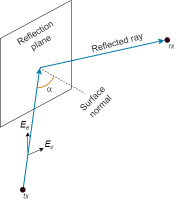
The model determines polarization and reflection loss using these steps.

1. Track the propagation of the ray in 3-D space by calculating the propagation matrix P. The matrix is a repeating product, where i is the number of reflection points.

   $$P={\displaystyle \prod _i{P}_i}$$

   For each reflection, calculate P_i by transforming the global coordinates of the incident electromagnetic field into the local coordinates of the reflection plane, multiplying the result by a reflection coefficient matrix, and transforming the coordinates back into the original global coordinate system [1]. The equations for P_i and P₀ are:

   $$P_i=\begin{array}{ccc}{\left[\begin{array}{ccc}{s}_{out}& p_{out}& k_{out}\end{array}\right]}_i& {\left[\begin{array}{ccc}{R}_V\left(\alpha \right)& 0& 0\\ 0& R_H\left(\alpha \right)& 0\\ 0& 0& 1\end{array}\right]}_i& {\left[\begin{array}{ccc}{s}_{in}& p_{in}& k_{in}\end{array}\right]}_i^{-1}\end{array}$$

   $$P_0=\left[\begin{array}{ccc}1& 0& 0\\ 0& 1& 0\\ 0& 0& 1\end{array}\right]$$

   where:

   • s, p, and k form a basis for the plane of incidence (the plane created by the incident ray and the surface normal of the reflection plane). s and p are perpendicular and parallel, respectively, to the plane of incidence.

   • k_in and k_out are the directions (in global coordinates) of the incident and exiting rays, respectively.

   • s_in and s_out are the directions (in global coordinates) of the horizontal polarizations for the incident and exiting rays, respectively.

   • p_in and p_out are the directions (in global coordinates) of the vertical polarizations for the incident and exiting rays, respectively.

   • R_H and R_V are the Fresnel reflection coefficients for the horizontal and vertical polarizations, respectively. α is the incident angle of the ray and ε_r is the complex relative permittivity of the material.

     $$R_H(\alpha )=\frac{\cos (\alpha )-\sqrt{({\epsilon }_r-{\sin }^2(\alpha ))/{\epsilon }_r{}^2}}{\cos (\alpha )+\sqrt{({\epsilon }_r-{\sin }^2(\alpha ))/{\epsilon }_r{}^2}}$$

     $$R_V(\alpha )=\frac{\cos (\alpha )-\sqrt{{\epsilon }_r-{\sin }^2(\alpha )}}{\cos (\alpha )+\sqrt{{\epsilon }_r-{\sin }^2(\alpha )}}$$

2. Project the propagation matrix P into a 2-by-2 polarization matrix R. The model rotates the coordinate systems for the transmitter and receiver so that they are in global coordinates.

   $$R=\left[\begin{array}{cc}{H}_{in}\cdot H_{rx}& V_{in}\cdot H_{rx}\\ H_{in}\cdot V_{rx}& V_{in}\cdot V_{rx}\end{array}\right]$$

   $$H_{in}=P(V_{tx}\times k_{tx})$$

   $$V_{in}=P{V}_{tx}$$

   where:

   • H_rx and V_rx are the directions (in global coordinates) of the horizontal (E_θ) and vertical (E_ϕ) polarizations, respectively, for the receiver.

   • H_in and V_in are the directions (in global coordinates) of the propagated horizontal and vertical polarizations, respectively.

   • V_tx is the direction (in global coordinates) of the nominal vertical polarization for the ray departing the transmitter.

   • k_tx is the direction (in global coordinates) of the ray departing the transmitter.

3. Specify the normalized horizontal and vertical polarizations of the electric field at the transmitter and receiver by using the 2-by-1 Jones polarization vectors J_tx and J_rx, respectively. If either the transmitter or receiver are unpolarized, then the model assumes $$J_{tx}=J_{rx}=\frac{\sqrt{2}}{2}\left[\begin{array}{c}1\\ 1\end{array}\right]$$.

4. Calculate the polarization and reflection loss IL by combining R, J_tx, and J_rx.

   $$IL=-20{\log }_{10}\left|J_{rx}^{-1}R{J}_{tx}\right|$$

Jones Vector Notation

For Jones vector notation, the raypl function describes signal polarization using Jones calculus.

The orthogonal components of Jones vectors are defined for E_θ and E_φ. This table shows the Jones vector corresponding to various antenna polarizations.

Antenna Polarization Type	Corresponding Jones Vector
Linear polarized in the θ direction	$$\left(\begin{array}{c}H\\ V\end{array}\right)=\left(\begin{array}{c}0\\ 1\end{array}\right)$$
Linear polarized in the φ direction	$$\left(\begin{array}{c}H\\ V\end{array}\right)=\left(\begin{array}{c}1\\ 0\end{array}\right)$$
Left-hand circular polarized (LHCP)	$$\left(\begin{array}{c}H\\ V\end{array}\right)=\frac{1}{\sqrt{2}}\left(\begin{array}{c}j\\ 1\end{array}\right)$$
Right-hand circular polarized (RHCP)	$$\left(\begin{array}{c}H\\ V\end{array}\right)=\frac{1}{\sqrt{2}}\left(\begin{array}{c}-j\\ 1\end{array}\right)$$

References

[1] Chipman, Russell A., Garam Young, and Wai Sze Tiffany Lam. "Fresnel Equations." In Polarized Light and Optical Systems. Optical Sciences and Applications of Light. Boca Raton: Taylor & Francis, CRC Press, 2019.

[2] International Telecommunications Union Radiocommunication Sector. Effects of building materials and structures on radiowave propagation above about 100MHz. Recommendation P.2040-1. ITU-R, approved July 29, 2015. https://www.itu.int/rec/R-REC-P.2040/en.

[3] International Telecommunications Union Radiocommunication Sector. Attenuation by atmospheric gases. Recommendation P.676-11. ITU-R, approved September 30, 2016. https://www.itu.int/rec/R-REC-P.676/en.

Extended Capabilities

C/C++ Code Generation

Generate C and C++ code using MATLAB® Coder™.

Usage notes and limitations:

When you specify multiple reflective materials, you must define each value as a character vector (char data type) in a cell array.

Version History

Introduced in R2020a

R2022b: Ray tracing models using SBR method find paths with exact geometric accuracy

When you find propagation paths using the raytrace function and a ray tracing model that uses the shooting and bouncing rays (SBR) method, MATLAB^® corrects the results so that the geometric accuracy of each path is exact, using single-precision floating-point computations. In previous releases, the paths have approximate geometric accuracy.

As a result, when you use rays returned by the raytrace function as input to the raypl function, the raypl function can return different results than in previous releases.