Room Impulse Response Simulation with Stochastic Ray Tracing
Room impulse response simulation aims to model the reverberant properties of a space without having to perform acoustic measurements. Many geometric and wave-based room acoustic simulation methods exist in the literature [1].
The image-source method is a popular geometric method (for an example, see Room Impulse Response Simulation with the Image-Source Method and HRTF Interpolation). One drawback of the image-source method is that it only models specular reflections between a transmitter and a receiver. There are other geometric methods that address this limitation by also taking sound diffusion into account. Stochastic ray tracing is one such method.
First, this example shows how to use acousticRoomResponse to perform stochastic ray tracing in a room in one line of code. Then, the example showcases the stochastic ray tracing algorithm step by step for a simple "shoebox" (cuboid) room.
Use acousticRoomResponse to Perform Acoustic Ray Tracing
Synthesize Impulse Response of Shoebox Room
Start with performing ray tracing on a shoebox room with acousticRoomResponse.
Define Room
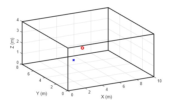
Define the room dimensions, in meters (width, length, and height, respectively).
roomDimensions = [10 8 4];
Treat the transmitter and receiver as points within the space of the room.
tx = [2 2 2];
rx = [5 5 1.8];
Plot the room space along with the receiver (red circle) and transmitter (blue x).
h = figure;
plotRoom(roomDimensions,rx,tx,h)

Define Reflection and Scattering Coefficients
A sound ray is reflected when it hits a surface. The reflection is a combination of a specular component and a diffused component. The relative strength of each component is determined by the reflection and scattering coefficients of the surfaces.
Define the absorption coefficients of the walls. The absorption coefficient is a measure of how much sound is absorbed (rather than reflected) when hitting a surface.
The frequency-dependent absorption coefficients are defined at the frequencies in the variable FVect [4]. In this section, you use the same coefficients for all walls in the room.
FVect = [125 250 500 1000 2000 4000 8000];
A = [.02 .02 .03 .03 .04 .05 .05];
Define the frequency-dependent scattering coefficients [5]. The scattering coefficient is defined as one minus the ratio between the specular reflected acoustic energy and the total reflected acoustic energy. In this section, you use the same coefficients for all walls in the room.
D = [.13 .56 .95 .95 .95 .95 0.95];
Synthesize Impulse Response
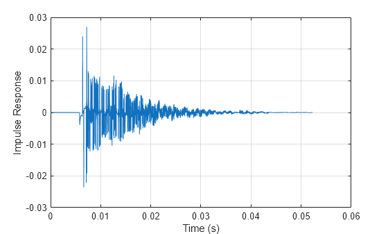
Synthesize and plot the impulse response using acousticRoomResponse. Specify the algorithm as "stochastic ray tracing". Use a sampling rate of 44.1 kHz.
fs = 44.1e3;
ir = acousticRoomResponse(roomDimensions,tx,rx,...
                          SampleRate=fs,...
                          Algorithm="stochastic ray tracing",...
                          BandCenterFrequencies=FVect,...
                          MaterialAbsorption=A,...
                          MaterialScattering=D);
figure
plot((1/fs)*(0:numel(ir)-1),ir)
grid on
xlabel("Time (s)")
ylabel("Impulse Response")

Auralize
Apply the synthesized impulse response to an audio signal.
[audioIn,fs] = audioread("FunkyDrums-44p1-stereo-25secs.mp3");
audioIn = audioIn(:,1);
Simulate the received audio by filtering with the impulse response.
audioOut = filter(ir,1,audioIn);
audioOut = audioOut/max(audioOut);
Listen to a few seconds of the original audio.
T = 10;
sound(audioIn(1:T*fs),fs)
pause(T)
Listen to a few seconds of the received audio.
sound(audioOut(1:T*fs),fs)
pause(T)
Synthesize Impulse Response of Non-Shoebox Room
Synthesize the impulse response of a more complex, non-shoebox room.
3-D model information is often stored in stereolithography (STL) files.
Load the room setup from a sample STL file.
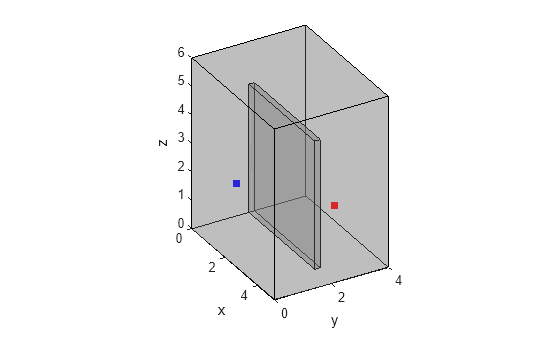
room = stlread("room.stl");Visualize the room along with the source and receiver positions. Notice that the room includes a partition wall. In this example, there is no line-of-sight between the transmitter and the receiver.
tx = [1 1 1.8];
rx = [3.5 3 1.7];
figure
visualizeGeneralRoom(room,tx,rx)

Synthesize the impulse response using acousticRoomResponse.
ir = acousticRoomResponse(room,tx,rx,...
                          SampleRate=fs,...
                          Algorithm="stochastic ray tracing",...
                          BandCenterFrequencies=FVect,...
                          MaterialAbsorption=A,...
                          MaterialScattering=D);
figure
plot((1/fs)*(0:numel(ir)-1),ir)
grid on
xlabel("Time (s)")
ylabel("Impulse Response")

Simulate the received audio by filtering with the impulse response.
audioOut = filter(ir,1,audioIn);
audioOut = audioOut/max(audioOut);
Listen to a few seconds of the received audio.
sound(audioOut(1:T*fs),fs)
pause(T)
Construct Room with Triangulation Objects
In the previous section, you loaded a room from an STL file.
You can also construct a custom room with triangulation objects. You can assign different custom material characteristics to each wall or section in the room.
Start with the room exterior.
roomDimensions = [5 4 6];

X = roomDimensions(1);
Y = roomDimensions(2);
Z = roomDimensions(3);

pts = [0 0 0;
       X 0 0;
       0 Y 0;
       X Y 0;
       0 0 Z;
       0 Y Z;
       X 0 Z;
       X Y Z];

dt = delaunayTriangulation(pts(:,1), pts(:,2), pts(:,3));
[conn, verts] = freeBoundary(dt);
Define the absorption and scattering coefficients of the room. Use the same coefficients for all the walls in the room.
roomAbsorption = repmat([0.02 0.02 0.03 0.03 0.04 0.05 0.05],12,1);
roomScattering = repmat([.01 .28 .7 .7 .74 .5 .5],12,1);
Next, design a partition wall in the room.
wallDimensions = [4 .2 4.5];

X = wallDimensions(1);
Y = wallDimensions(2);
Z = wallDimensions(3);

pts = [0 0 0;
       X 0 0;
       0 Y 0;
       X Y 0;
       0 0 Z;
       0 Y Z;
       X 0 Z;
       X Y Z] + [0 2 0];

dt2 = delaunayTriangulation(pts(:,1), pts(:,2), pts(:,3));
[conn2, verts2] = freeBoundary(dt2);
conn2 = conn2 + size(verts,1);
Define the absorption and scattering coefficients of the partition wall.
wallAbsorption = repmat([0.02 0.03 0.04 0.05 0.04 0.03 0.02],12,1);
wallScattering = repmat([.01 .28 .7 .7 .74 .5 .5],12,1);
Combine the room and the partition wall.
room = triangulation([conn;conn2],[verts;verts2])
room =
  triangulation with properties:

              Points: [16×3 double]
    ConnectivityList: [24×3 double]
Visualize the room using the helper function visualizeGeneralRoom.
visualizeGeneralRoom(room,tx,rx)
Combine the scattering and absorption coefficients of the room and the partition wall.
roomAbsorption = [roomAbsorption;wallAbsorption];
roomScattering = [roomScattering;wallScattering];
Synthesize and plot the impulse response of the room using acousticRoomResponse.
ir = acousticRoomResponse(room,tx,rx,...
                         Algorithm="stochastic ray tracing",...
                         BandCenterFrequencies=[125 250 500 1000 2000 4000 8000],...
                         MaterialAbsorption=roomAbsorption,...
                         MaterialScattering=roomScattering);
t = (0:numel(ir)-1)/fs;
figure
plot(t,ir)
grid on
xlabel("Time (s)")
ylabel("Impulse Response")
Simulate the received audio by filtering with the impulse response.
audioOut = filter(ir,1,audioIn);
audioOut = audioOut/max(audioOut);
Listen to a few seconds of the received audio.
sound(audioOut(1:T*fs),fs)
Stochastic Ray Tracing Algorithm
In this section, you learn how acousticRoomResponse operates by implementing the ray tracing algorithm step-by-step. For simplicity, you use a simple shoebox room.
Ray tracing assumes that sound energy travels around the room in rays. The rays start at the sound source, and are emitted in all directions, following a uniform random distribution. In this section, you follow (trace) rays as they bounce off obstacles (walls, floor and ceiling) in the room. You treat each ray wall incidence point as a secondary source which transmits some of its energy to the receiver. You use this energy to update a frequency-dependent histogram. You then compute the room impulse response by weighting a Poisson random process by the histogram values [2].
Define Room
Define the room dimensions, in meters (width, length, and height, respectively).
roomDimensions = [10 8 4];
Define the transmitter and receiver locations. Assume that the receiver is a sphere with radius 8.75 cm.
tx = [2 2 2];
rx = [5 5 1.8];
r = 0.0875;
Plot the room space along with the receiver (red circle) and transmitter (blue x).
h = figure;
plotRoom(roomDimensions,rx,tx,h)
Define Reflection and Scattering Coefficients
Define the absorption coefficients of the walls. Each row represents the coefficient of an individual wall.
FVect = [125 250 500 1000 2000 4000 8000];
A = [.02, .02, .03, .03, .04, .05, .05;
    .02, .02, .03, .03, .03, .04, .04;
    .02, .02, .03, .03, .04, .07, .07;
    .02, .02, .03, .03, .04, .05, .05;
    .02, .02, .03, .03, .04, .05, .05;
    .02, .02, .03, .03, .04, .05, .05];
Derive the reflection coefficients of the six surfaces from the absorption coefficients.
R = 1-A;
Define the frequency-dependent scattering coefficients . Each row represents the coefficient of an individual wall.
D = [.13, .56, .95, .95, .95, .95, 0.95;
    .5, .9, .95, .95, .95, .95, 0.95;
    .5, .9, .95, .95, .95, .95, 0.95;
    .13, .56, .95, .95, .95, .95, 0.95;
    .13, .56, .95, .95, .95, .95, 0.95;
    .13, .56, .95, .95, .95, .95, 0.95];
Generate Random Rays
First, generate rays emanating from the source in random directions.
Set the number of rays.
N = 5000;
Generate the rays using the helper function RandSampleSphere. rays is a N-by-3 matrix. Each row of rays holds the three-dimensional ray vector direction.
rng(0)
rays = RandSampleSphere(N);
size(rays)
ans = 1×2

        5000           3
Initialize Energy Histogram
As you trace the rays, you update a two-dimensional histogram of the energy detected at the receiver. The histogram records values along time and frequency.
Set the histogram time resolution, in seconds. The time resolution is typically much larger than the inverse of the audio sample rate.
histTimeStep = 0.0040;
Compute the number of histogram time bins. In this example, limit the impulse response length to half a second.
impResTime = 0.5;
nTBins = round(impResTime/histTimeStep);
The ray tracing algorithm is frequency-selective. In this example, focus on six frequency bands, centered around the frequencies in FVect.
The number of frequency bins in the histogram is equal to the number of frequency bands.
nFBins = length(FVect);
Initialize the histogram.
TFHist = zeros(nTBins,nFBins);
Perform Ray Tracing
Compute the received energy histogram by tracing the rays over each frequency band. When a ray hits a surface, record the amount of diffused ray energy seen at the receiver based on the diffused rain model [2]. The new ray direction upon hitting a surface is a combination of a specular reflection and a random reflection. Continue tracing the ray until its travel time exceeds the impulse response duration.
for iBand = 1:nFBins
    % Perform ray tracing independently for each frequency band.
    for iRay = 1:size(rays,1)
        % Select ray direction
        ray = rays(iRay,:);
        % All rays start at the source/transmitter
        ray_xyz = tx;
        % Set initial ray direction. This direction changes as the ray is
        % reflected off surfaces.
        ray_dxyz = ray;
        % Initialize ray travel time. Ray tracing is terminated when the
        % travel time exceeds the impulse response length.
        ray_time = 0;
        % Initialize the ray energy. Energy decreases when the ray hits
        % a surface.
        ray_energy = 1/size(rays,1);

        while (ray_time <= impResTime)

            % Determine the surface that the ray encounters
            [surfaceofimpact,displacement] = getImpactWall(ray_xyz,...
                                             ray_dxyz,roomDimensions);

            % Determine the distance traveled by the ray
            distance = sqrt(sum(displacement.^2));

            % Determine the coordinates of the impact point
            impactCoord = ray_xyz+displacement;

            % Update ray location/source
            ray_xyz = impactCoord;

            % Update cumulative ray travel time
            c = 343; % speed of light (m/s)
            ray_time = ray_time+distance/c;

            % Apply surface reflection to ray's energy
            % This is the amount of energy that is not lost through
            % absorption.
            ray_energy = ray_energy*R(surfaceofimpact,iBand);

            % Apply diffuse reflection to ray energy
            % This is the fraction of energy used to determine what is
            % detected at the receiver
            rayrecv_energy = ray_energy*D(surfaceofimpact,iBand);

            % Adjust the amount of reflected energy
            ray_energy = ray_energy * (1-D(surfaceofimpact,iBand));

            % Determine impact point-to-receiver direction.
            rayrecvvector = rx-impactCoord;

            % Determine the ray's time of arrival at receiver.
            distance = sqrt(sum(rayrecvvector.*rayrecvvector));
            recv_timeofarrival = ray_time+distance/c;

            if recv_timeofarrival>impResTime
                break
            end

            % Determine amount of diffuse energy that reaches the receiver.
            % See (5.20) in [2].

            % Compute received energy
            N = getWallNormalVector(surfaceofimpact);
            cosTheta = sum(rayrecvvector.*N)/(sqrt(sum(rayrecvvector.^2)));
            cosAlpha = sqrt(sum(rayrecvvector.^2)-r^2)/sqrt(sum(rayrecvvector.^2));
            E = (1-cosAlpha)*2*cosTheta*rayrecv_energy;

            % Scale the energy by the traveled distance
            E = E/(recv_timeofarrival*c)^2;

            % Update energy histogram
            tbin = floor(recv_timeofarrival/histTimeStep + 0.5);
            TFHist(tbin,iBand) = TFHist(tbin,iBand) + E;

            % Compute a new direction for the ray.
            % Pick a random direction that is in the hemisphere of the
            % normal to the impact surface.
            d = rand(1,3);
            d = d/norm(d);
            if sum(d.*N)<0
                d = -d;
            end

            % Derive the specular reflection with respect to the incident
            % wall
            ref = ray_dxyz-2*(sum(ray_dxyz.*N))*N;

            % Combine the specular and random components
            d = d/norm(d);
            ref = ref/norm(ref);
            ray_dxyz = D(surfaceofimpact,iBand)*d+(1-D(surfaceofimpact,iBand))*ref;
            ray_dxyz = ray_dxyz/norm(ray_dxyz);
        end
    end
end
View Energy Histogram
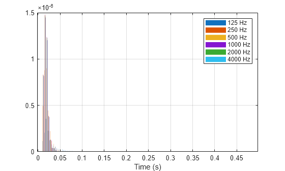
Plot the computed frequency-dependent histogram.
figure
bar(histTimeStep*(0:size(TFHist,1)-1),TFHist)
grid on
xlabel("Time (s)")
legend(["125 Hz","250 Hz","500 Hz","1000 Hz","2000 Hz","4000 Hz"])
Generate Room Impulse Response
The energy histogram represents the envelope of the room impulse response. Synthesize the impulse response using a Poisson-distributed noise process [2].
Generate Poisson Random Process
You model sound reflections as a Poisson random process.
Define the start time of the process.
V = prod(roomDimensions);
t0 = ((2*V*log(2))/(4*pi*c^3))^(1/3); % eq 5.45 in [2]
Initialize the random process vector and the vector containing the times at which events occur.
poissonProcess = [];
timeValues = [];
Create the random process.
t = t0;
while (t<impResTime)
    timeValues = [timeValues t]; %#ok
    % Determine polarity.
    if (round(t*fs)-t*fs) < 0
        poissonProcess = [poissonProcess 1]; %#ok
    else
        poissonProcess = [poissonProcess -1];%#ok
    end
    % Determine the mean event occurrence (eq 5.44 in [2])
    mu = min(1e4,4*pi*c^3*t^2/V);
    % Determine the interval size (eq. 5.44 in [2])
    deltaTA = (1/mu)*log(1/rand); % eq. 5.43 in [2])
    t = t+deltaTA;
end
Create a random process sampled at the specified sample rate.
randSeq = zeros(ceil(impResTime*fs),1);
for index=1:length(timeValues)
    randSeq(round(timeValues(index)*fs)) = poissonProcess(index);
end
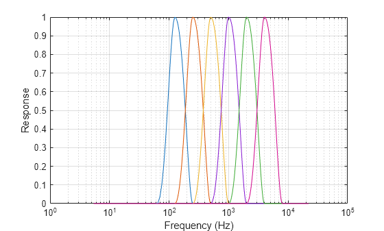
Pass Poisson Process Through Bandpass Filters
You create the impulse response by passing the Poisson process through bandpass filters centered at the frequencies in FVect, and then weighting the filtered signals with the received energy envelope computed in the histogram.
Define the lower and upper cutoff frequencies of the bandpass filters.
flow =  FVect/2;
fhigh = FVect*2;
Set the FFT length.
NFFT = 8192;
Get the frequency vector corresponding to the FFT values.
sfft = dsp.STFT(FFTLength=NFFT,FrequencyRange="onesided");
F = sfft.getFrequencyVector(fs);
Create the bandpass filters (use equation 5.46 in [2]).
RCF = zeros(length(FVect),length(F));
for index0 = 1:length(FVect)
    for index=1:length(F)
        f = F(index);
        if f<FVect(index0) && f>=flow(index0)
            RCF(index0,index) = .5*(1+cos(2*pi*f/FVect(index0)));
        end
        if f<fhigh(index0) && f>=FVect(index0)
            RCF(index0,index) = .5*(1-cos(2*pi*f/(2*FVect(index0))));
        end
    end
end
Plot the bandpass filter frequency responses.
figure
semilogx(F,RCF(1,:))
hold on
semilogx(F,RCF(2,:))
semilogx(F,RCF(3,:))
semilogx(F,RCF(4,:))
semilogx(F,RCF(5,:))
semilogx(F,RCF(6,:))
semilogx(F,RCF(6,:))
xlabel("Frequency (Hz)")
ylabel("Response")
grid on
RCF = fftshift(ifft(RCF,NFFT,2,'symmetric'),2);Filter the Poisson sequence through the six bandpass filters.
y = zeros(length(randSeq),6);
for index=1:length(FVect)
    y(:,index) = conv(randSeq,RCF(index,:),'same');
end
Combine the Filtered Sequences
Construct the impulse response by weighting the filtered random sequences sample-wise using the envelope (histogram) values.
Compute the times corresponding to the impulse response samples.
impTimes = (1/fs)*(0:size(y,1)-1);
Compute the times corresponding to the histogram bins.
hisTimes = histTimeStep/2 + histTimeStep*(0:nTBins);
Compute the weighting factors (equation 5.47 in [2]).
W = zeros(size(impTimes,2),numel(FVect));
EdgeF = getBandedgeFrequencies(FVect,fs);
BW = diff(EdgeF);
for k=1:size(TFHist,1)
    gk0 = floor((k-1)*fs*histTimeStep)+1;
    gk1 = floor(k*fs*histTimeStep);
    yy = y(gk0:gk1,:).^2;
    val = sqrt(TFHist(k,:)./sum(yy,1)).*sqrt(BW/(fs/2));
    for iRay=gk0:gk1
        W(iRay,:)= val;
    end
end
Create the impulse response.
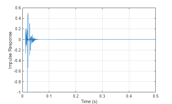
y = y.*W;
ip = sum(y,2);
ip = ip./max(abs(ip));
Auralization
Plot the impulse response.
figure
plot((1/fs)*(0:numel(ip)-1),ip)
grid on
xlabel("Time (s)")
ylabel("Impulse Response")
Apply the impulse response to an audio signal.
[audioIn,fs] = audioread("FunkyDrums-44p1-stereo-25secs.mp3");
audioIn = audioIn(:,1);
Simulate the received audio by filtering with the impulse response.
audioOut = filter(ip,1,audioIn);
audioOut = audioOut/max(audioOut);
Listen to a few seconds of the original audio.
T = 10;
sound(audioIn(1:T*fs),fs)
pause(T)
Listen to a few seconds of the received audio.
sound(audioOut(1:T*fs),fs)
References
[1] "Overview of geometrical room acoustic modeling techniques", Lauri Savioja, Journal of the Acoustical Society of America 138, 708 (2015).
[2] "Physically Based Real-Time Auralization of Interactive Virtual Environments", Dirk Schröder, Aachen, Techn. Hochsch., Diss., 2011.
[3] "Auralization: Fundamentals of Acoustics, Modelling, Simulation, Algorithms and Acoustic Virtual Reality", Michael Vorlander, Second Edition, Springer.
[4] https://www.acoustic.ua/st/web_absorption_data_eng.pdf
[5] "Scattering in Room Acoustics and Related Activities in ISO and AES", Jens Holger Rindel, 17th ICA Conference, Rome, Italy, September 2001.
Helper Functions
function plotRoom(roomDimensions,rx,tx,figHandle)
% PLOTROOM Helper function to plot 3D room with receiver/transmitter points
figure(figHandle)
X = [0;roomDimensions(1);roomDimensions(1);0;0];
Y = [0;0;roomDimensions(2);roomDimensions(2);0];
Z = [0;0;0;0;0];
figure;
hold on;
plot3(X,Y,Z,"k",LineWidth=1.5);
plot3(X,Y,Z+roomDimensions(3),"k",LineWidth=1.5);
set(gca,"View",[-28,35]);
for k=1:length(X)-1
    plot3([X(k);X(k)],[Y(k);Y(k)],[0;roomDimensions(3)],"k",LineWidth=1.5);
end
grid on
xlabel("X (m)")
ylabel("Y (m)")
zlabel("Z (m)")
plot3(tx(1),tx(2),tx(3),"bx",LineWidth=2)
plot3(rx(1),rx(2),rx(3),"ro",LineWidth=2)
end

function X=RandSampleSphere(N)
% RANDSAMPLESPHERE Return random ray directions

% Sample the unfolded right cylinder
z = 2*rand(N,1)-1;
lon = 2*pi*rand(N,1);

% Convert z to latitude
z(z<-1) = -1;
z(z>1) = 1;
lat = acos(z);

% Convert spherical to rectangular co-ords
s = sin(lat);
x = cos(lon).*s;
y = sin(lon).*s;

X = [x y z];
end

function [surfaceofimpact,displacement] = getImpactWall(ray_xyz,ray_dxyz,roomDims)
% GETIMPACTWALL Determine which wall the ray encounters
surfaceofimpact = -1;
displacement = 1000;
%  Compute time to intersection with x-surfaces
if (ray_dxyz(1) < 0)
    displacement = -ray_xyz(1) / ray_dxyz(1);
    if displacement==0
        displacement=1000;
    end
    surfaceofimpact = 0;
elseif (ray_dxyz(1) > 0)
    displacement = (roomDims(1) - ray_xyz(1)) / ray_dxyz(1);
    if displacement==0
        displacement=1000;
    end
    surfaceofimpact = 1;
end
% Compute time to intersection with y-surfaces
if ray_dxyz(2)<0
    t = -ray_xyz(2) / ray_dxyz(2);
    if (t<displacement) && t>0
        surfaceofimpact = 2;
        displacement = t;
    end
elseif ray_dxyz(2)>0
    t = (roomDims(2) - ray_xyz(2)) / ray_dxyz(2);
    if (t<displacement) && t>0
        surfaceofimpact = 3;
        displacement = t;
    end
end
% Compute time to intersection with z-surfaces
if ray_dxyz(3)<0
    t = -ray_xyz(3) / ray_dxyz(3);
    if (t<displacement) && t>0
        surfaceofimpact = 4;
        displacement = t;
    end
elseif ray_dxyz(3)>0
    t = (roomDims(3) - ray_xyz(3)) / ray_dxyz(3);
    if (t<displacement) && t>0
        surfaceofimpact = 5;
        displacement = t;
    end
end
surfaceofimpact = surfaceofimpact + 1;

displacement = displacement * ray_dxyz;

end

function N = getWallNormalVector(surfaceofimpact)
% GETWALLNORMALVECTOR Get the normal vector of a surface
switch surfaceofimpact
    case 1
        N = [1 0 0];
    case 2
        N = [-1 0 0];
    case 3
        N = [0 1 0];
    case 4
        N = [0 -1 0];
    case 5
        N = [0 0 1];
    case 6
        N = [0 0 -1];
end

end

function bef = getBandedgeFrequencies(cf,fs)
G = 2;
BandsPerOctave = 1;
fbpo = .5/BandsPerOctave;
bef = [ cf(1)*G^-fbpo, ...
    sqrt(cf(1:end-1).*cf(2:end)), ...
    min(cf(end)*G^fbpo, fs/2) ];
end

function visualizeGeneralRoom(tri,txinates,rxinates)
figure;
trisurf(tri, ...
    'FaceAlpha', 0.3, ...
    'FaceColor', [.5 .5 .5], ...
    'EdgeColor', 'none');
view(60, 30);
hold on; axis equal; grid off;
xlabel('x'); ylabel('y'); zlabel('z');
% Plot edges
fe = featureEdges(tri,pi/20);
numEdges = size(fe, 1);
pts = tri.Points;
a = pts(fe(:,1),:);
b = pts(fe(:,2),:);
fePts = cat(1, reshape(a, 1, numEdges, 3), ...
           reshape(b, 1, numEdges, 3), ...
           nan(1, numEdges, 3));
fePts = reshape(fePts, [], 3);
plot3(fePts(:, 1), fePts(:, 2), fePts(:, 3), 'k', 'LineWidth', .5);

hold on
tx = txinates;
rx = rxinates;
scatter3(tx(1), tx(2), tx(3), 'sb', 'filled');
scatter3(rx(1,1), rx(1,2), rx(1,3), 'sr', 'filled');
end