visualize
Visualize and validate filter response
Description
visualize( plots the
magnitude response of the frequency-weighted filter weightFilt)weightFilt.
The plot is updated automatically when properties of the object change.
visualize(
uses an weightFilt,N)N-point FFT to calculate the magnitude response.
visualize(___, creates
a mask based on the class of filter specified by mType)mType, using
either of the previous syntaxes.
hvsz = visualize(___)dsp.DynamicFilterVisualizer object when called with any of the
previous syntaxes.
Examples
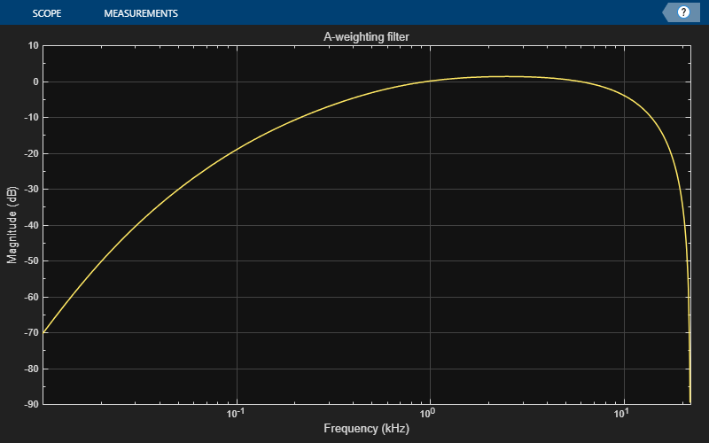
Create a weightingFilter System object™ and then plot the magnitude response of the filter.
weightFilt = weightingFilter;
visualize(weightFilt)
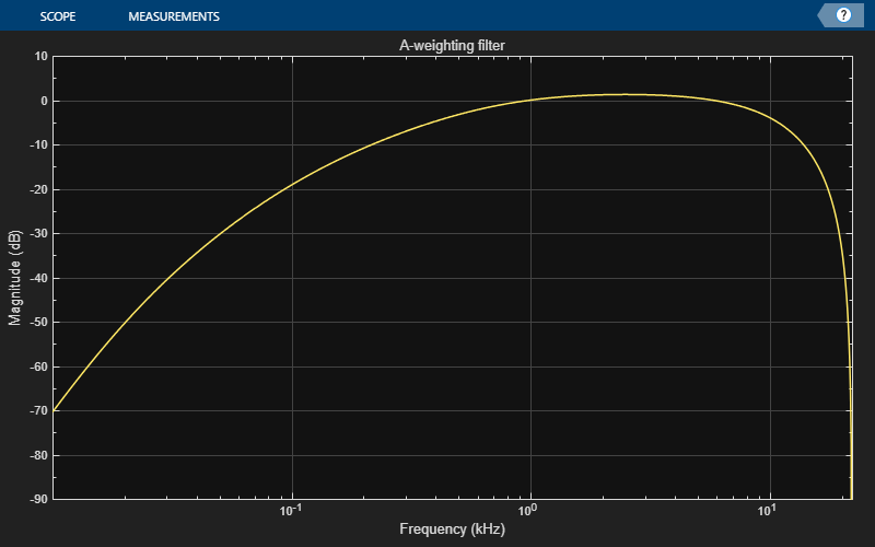
Create a weightingFilter System object™. Plot a 1024-point frequency representation.
weightFilt = weightingFilter;
visualize(weightFilt,1024)
Create a weightingFilter System object™. Visualize the class 2 compliance of the filter design.
weightFilt = weightingFilter;
visualize(weightFilt,'class 2')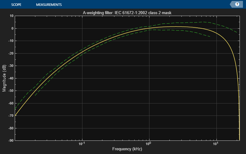
Input Arguments
Version History
Introduced in R2016b