Designing for Reliability and Robustness
By Stuart Kozola, MathWorks
No design is free from uncertainty or natural variation. For example, how will the design be used? How will it respond to environmental factors or to changes in manufacturing or operational processes? These kinds of uncertainty compound the challenge of creating designs that are reliable and robust –designs that perform as expected over time and are insensitive to changes in manufacturing, operational, or environmental factors.
Using an automotive suspension system as an example, this article describes tools and techniques in MATLAB®, Statistics and Machine Learning Toolbox™, and Optimization Toolbox™ software that let you extend a traditional design optimization approach to account for uncertainty in your design, improving quality and reducing prototype testing and overall development effort.
We begin by designing a suspension system that minimizes the forces experienced by front- and rear-seat passengers when the automobile travels over a bump in the road. We then modify the design to account for suspension system reliability; we want to ensure that the suspension system will perform well for at least 100,000 miles. We conclude our analysis by verifying that the design is resilient to, or unaffected by, changes in cargo and passenger mass.
Performing Traditional Design Optimization
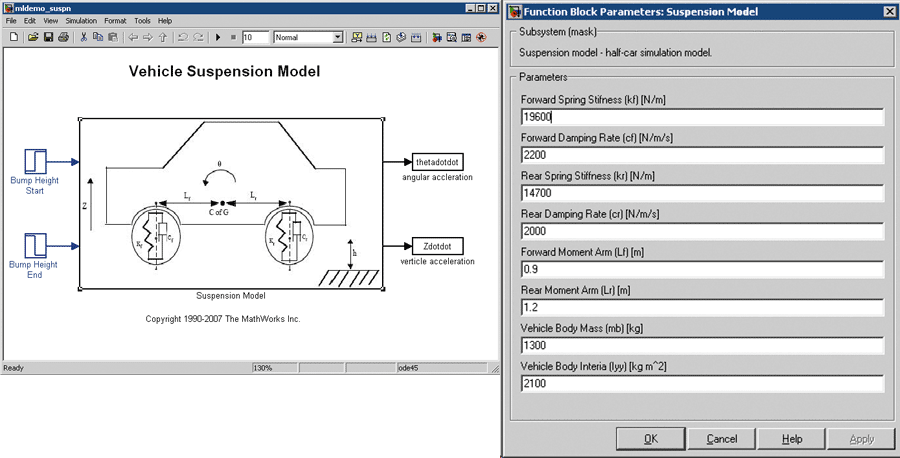
Our Simulink suspension system model (Figure 1) has two inputs – the bump starting and ending height – and eight adjustable parameters. We can modify the four parameters that define the front and rear suspension system stiffness and damping rate: kf, kr, cf, cr. The remaining parameters are defined by applying passenger and cargo loading to the vehicle, and are not considered to be design parameters.
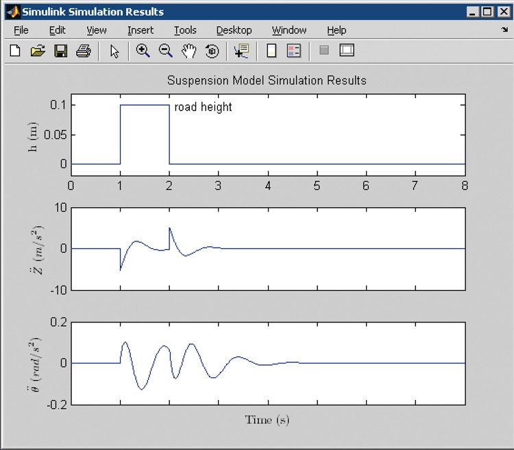
The model outputs are angular acceleration about the center of gravity (thetadotddot,IMAGE) and vertical acceleration (zdotdot,IMAGE). Figure 2 illustrates the model response for our initial design to a simulated bump in the road.
Our goal is to set the parameters kf, kr, cf, and cr to minimize the discomfort that front- and rear-seat passengers experience as a result of traveling over a bump in the road. We use acceleration as a proxy for passenger discomfort. The design optimization problem can be summarized as follows:
| Objective: | Minimize peak and total acceleration |
| Design variables: | Front/rear spring/shock absorber design (kr, kr, cf, cr) |
| Design constraints: | Car is level when at rest. Suspension system maintains a natural frequency of vibration below 2 Hz. Damping ratio remains between 0.3 and 0.5. |
This problem is nonlinear in both response (Figure 2) and design constraints. To solve it, a nonlinear optimization solver is required. The Optimization Toolbox solver fmincon is designed specifically for this type of problem.
We begin by casting our optimization problem into the form accepted by fmincon. The table below summarizes the problem formulation that fmincon accepts and the definition of the suspension problem in MATLAB syntax.
|
Suspension Problem (MATLAB M-code) |
|
|---|---|---|
Objective |
\(\min_{x} f(x)\) |
|
Design variables |
\(x\) |
x = [kf, cf, kr, cr] |
Nonlinear constraints |
\(c(x) \leq 0\) |
|
Linear constraints |
\(A \cdot x \leq b\) |
A = []; % none for this problem |
Bound constraints |
\(lb \leq x \leq ub\) |
lb = [10000; 100; 10000; 100]; |
The design objective is defined as an M-file function myCostFcn that accepts two inputs: the design vector x and simParms (Figure 3). x contains our design variables for the suspension system. simParms is a structure that passes in the remaining defining parameters of the Simulink model(Mb, Lf, Lr, and Iyy). myCostFcn runs the suspension model defined by x and simParms and returns a measure of passenger discomfort, calculated as the weighted average of the peak and total acceleration, as shown in Figure 3. Passenger discomfort is normalized so that our initial design has a discomfort level of 1.
Nonlinear constraints are defined in the M-file function mynonlcon that returns values for c(x) and ceq(x). The linear and bound constraints are defined as shown in the table as constant coefficient matrices (A, Aeq) or vectors (b, beq, lb, ub).
Figure 3 shows our problem defined and solved using the Optimization Tool graphical user interface (optimtool), which simplifies the tasks of defining an optimization problem, choosing an appropriate solver, setting solver options, and running the solver.
Using a traditional optimization approach, we found that the optimal design was one where x = [kf, cf, kr, cr] = [13333, 2225, 10000, 1927].
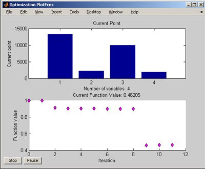
Figure 4 shows a standard Optimization Toolbox solution progress plot. The top plot shows the current value of the design variables for the current solver iteration, which at iteration 11 is the final solution. The bottom plot shows the objective function value (passenger discomfort relative to the initial design) across solver iterations. This plot shows that our initial design (iteration 0) had a discomfort level of 1, while the optimal design, found after 11 iterations, has a discomfort level of 0.46 – a reduction of 54% from our initial design.
Ensuring Suspension System Reliability
Our optimal design satisfies the design constraints, but is it a reliable design? Will it perform as expected over a given time period? We want to ensure that our suspension design will perform as intended for at least 100,000 miles.
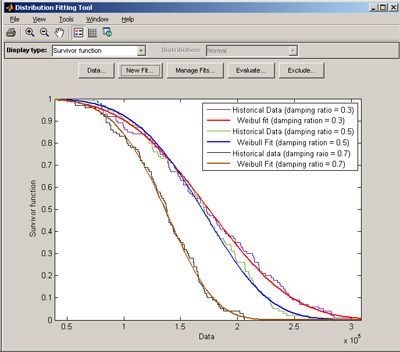
To estimate the suspension's reliability, we use historical maintenance data for similar suspension system designs (Figure 5). The horizontal axis represents the driving time, reported as miles. The vertical axis shows how many suspension systems had degraded performance requiring repair or servicing. The different sets of data apply to suspension systems with different damping ratios. The damping ratio is defined as
\[\eta = \frac{c}{2\sqrt{kM}}\]
where c is the damping coefficient (cf or cr), k is the spring stiffness (kf or kr), and M is the amount of mass supported by the front or rear suspension. The damping ratio is a measure of the stiffness of the suspension system.
We fit Weibull distributions to the historical data using the Distribution Fitting Tool (dfittool). Each fit provides a probability model that we can use to predict our suspension system reliability as a function of miles driven. Collectively, the three Weibull fits let us predict how the damping ratio affects the suspension system reliability as a function of miles driven. For example, the optimal design found previously has a damping ratio for the front and rear suspension of 0.5. Using the plots in Figure 5, we can expect that after 100,000 miles of operation, our design will have 88% of the original designs operating without the need for repair. Conversely, 12% of the original designs will require repair before 100,000 miles.
We want to improve our design so that it has a 90% survival rate at 100,000 miles of operation. We add this reliability constraint to our traditional optimization problem by adding a nonlinear constraint to mynonlcon.
Plimit = 0.90;              % maximum probability of shock absorber failure
A  = @(dampRatio) -1.0129e+005.*dampRatio.^2 -28805.*dampRatio + 2.1831e+005;
B  = @(dampRatio) 1.6865.*dampRatio.^2 -1.8534.*dampRatio + 4.1507;
Ps = @(miles, dampRatio) 1 - wblcdf(miles, A(dampRatio), B(dampRatio));

% Add inequality constraint to existing constraints
c = [c;              % keep original constraints
Plimit- Ps(cdf, Mileage);...     % front reliability constraint
Plimit- Ps(cdr, Mileage)];       % rear reliability constraint
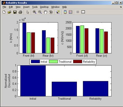
We solve the optimization problem as before using optimtool. The results, summarized in Figure 6, show that including the reliability constraint changed the design values for cf and cr and resulted in a slightly higher discomfort level. The reliability-based design still performs better than the initial design.
Optimizing for Robustness
Our design is now reliable—it meets our life and design goals—but it may not be robust. Operation of the suspension-system design is affected by changes in the mass distribution of the passengers or cargo loads. To be robust, the design must be insensitive to changes in mass distribution.
To account for a distribution of mass loadings in our design, we use Monte Carlo simulation, repeatedly running the Simulink model for a wide range of mass loadings at a given design. The Monte Carlo simulation will result in the model output having a distribution of values for a given set of design variables. The objective of our optimization problem is therefore to minimize the mean and standard deviation of passenger discomfort.
We replace the single simulation call in myCostFcn with the Monte Carlo simulation and optimize for the set of design values that minimize the mean and standard deviation of total passenger discomfort. We’ll assume that the mass distribution of passengers and trunk loads follow Rayleigh distributions and randomly sample the distributions to define conditions to test our design performance.
nRuns = 10000;
front = 40 + raylrnd(40, nRuns, 1);   % front passengers - adults (kg)
back = 1.36 + raylrnd(40, nRuns, 1);  % rear passengers – includes children
trunk = raylrnd(10, nRuns, 1);    % additional mass for luggage (kg)
The total mass, center of gravity, and moment of inertia are adjusted to account for the changes in mass distribution of the automobile.
mcMb = Mb + front + back + trunk; % total mass
mcCm = (front.*rf - back.*rr - trunk.*rt)./mcMb; % update center of mass
% Adjust moment of inertia
mcIyy = Iyy + front.*rf.^2 + back.*rr.^2 + trunk.*rt.^2- mcMb.*mcCm.^2;
The optimization problem, including the reliability constraints, is solved as before in optimtool. The results are shown in Figure 7. The robust design has an average discomfort level that is higher than that in the reliability-based design, resulting in a design with higher damping coefficient values.
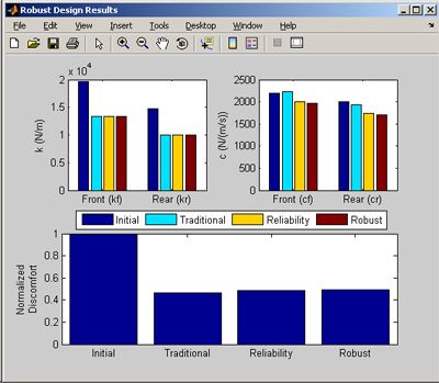
The discomfort measure reported in Figure 7 is an average value for the robust design case. Figure 8 displays a scatter-matrix plot that summarizes variability seen in discomfort as a result of different mass loadings for the robust design case.
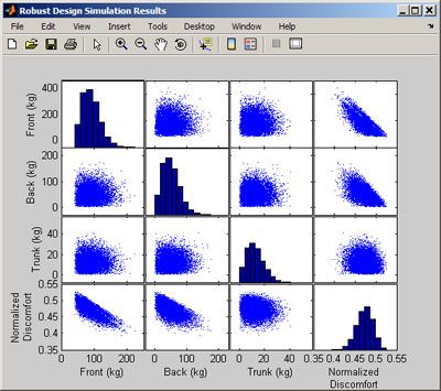
The diagonals show a histogram of the variables listed on the axis. The plots above and below the diagonal are useful for quickly finding trends across variables. The histograms for front, back, and trunk represent the distribution of the inputs to our simulation. The histogram for discomfort shows that it is concentrated around the value 0.47 and is approximately normally distributed. The plots below the diagonal do not show a strong trend in discomfort with trunk loading levels, indicating that our design is robust to changes in this parameter. There is a definite trend associated with the front loading on discomfort. Front loading appears to be approximately linear with a min of 0.43 and a max of 0.52. A trend between back loading and discomfort can also be seen, but from this plot it is difficult determine if it is linear. From this plot, it is difficult to determine whether our design is robust with respect to back loading.
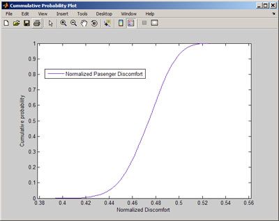
Using a cumulative probability plot of the discomfort results (Figure 9), we estimate that 90% of the time, passengers will experience less than 50% of the discomfort they would have experienced with the initial design. We can also see that our new design maintains a normalized level of discomfort below 0.52 nearly 100% of the time. We therefore conclude that our optimized design overall is robust to expected variation in loadings and will perform better than our initial design.
Design Trade-Offs
This article showed how MATLAB, Statistics and Machine Learning Toolbox, and Optimization Toolbox can be used to capture uncertainty within a simulation-based design problem in order to find an optimal suspension design that is reliable and robust.
We began by showing how to reformulate a design problem as an optimization problem that resulted in a design that performed better than the initial design. We then modified the optimization problem to include a reliability constraint. The results showed that a trade-off in performance was required to meet our reliability goals.
We completed our analysis by including the uncertainty that we would expect to see in the mass loading of the automobile. The results showed that we derived a different design if we accounted for uncertainty in operation and quantified the expected variability in performance. The final design traded performance to maintain reliability and robustness.
Published 2008 - 91545v00
