I Need Results Yesterday: Accelerating Your Wireless Communications Simulations

Hi, my name is Mike McLernon and I'm here to talk to you about a topic that is probably very, very pervasively interesting to a lot of people, and that is about accelerating your wireless communications solutions. We've all heard the edict from our manager. We want results yesterday. We want our simulations to run faster. We need results. And I'm going to tell you about how you can accelerate those simulations. I've been with MathWorks since 2001 for many of those years in the development organization, building some of these communications capabilities, simulation capabilities that we're going to talk about. More recently, I have moved over to technical product marketing, and I'm here again to tell you how you can make your comm simulations faster.

So here's what we're going to talk about. There's a whole array of topics that we are going to cover. But the first thing that we're going to do is introduce and motivate the topic. So who wants their code to run slower? Typically, nobody. And you're probably experiencing this. Your design cycles are getting shorter, but the parameter spaces that you have to iterate over to get to an optimum design are getting broader and larger. Consider how many parameters go into a 5G system, hundreds, if not thousands.

Well, here we have an image of our favorite reptile, the tortoise. He's reputed to be slow, but he's steady. And here's his worthy nemesis, the rabbit, the hare. He's fast, but he doesn't really ever win the race. The fable goes that slow and steady wins the race. But in today's design world, fast and steady wins the race. You need reliable results and you need them fast.

So what are your options? The good news here is that you have many, many ways in which to accelerate your code. And we're going to talk about MATLAB. We're going to talk about local CPUs that might reside on your laptop or your desktop, a CPU cluster that your organization may have, GPUs that are getting more and more popular with each passing year, cloud computing, where you can leverage AWS or Azure to accelerate your simulations, and perhaps in the most extreme case, using FPGAs to really accelerate a certain part of your model.

But first, before we talk about any acceleration techniques, let's talk about measuring. Just like in construction, you want to measure twice and then cut once. If you arbitrarily look to accelerate a certain piece of your code that only occupies 1% of the full system time, you've wasted your time. First, you want to find out where the hotspots are and then you go ahead and address those tall poles. So this image here is an image of many, many apps that MATLAB has produced to accelerate your workflows. And in particular, inside the red box is a Profiler app.

I've been using the Profiler for roughly 20 years, and it has been one of the best things that is in MATLAB. It drills in immediately to find out where those sticking points are in your code, so that you can do something about it. So let's see it in action. So let's get out of slides, and actually we'll get into MATLAB. What we're going to do is run this code, and we're going to actually profile it. So I'm in the Editor right now and you can see-- let's see. We'll go to the Editor. There you go. The Profiler.

So if you're in the editor, you can click on this Profiler icon and then it brings up the Profiler app. So the code that you want to profile is already populated in this edit bar. So I'm just going to run it and time it. So this takes a little bit of time. So let's walk through the actual code that we're running. So it is a BER simulation. This is a bread and butter type application for any wireless engineer. And BER simulations are very, very easily accelerated.

So here's what we do. We decide what our Eb/N0 range is. We decide how many errors we're going to collect. And then we go ahead and run a simulation in an Eb/N0 loop. And let's take a look at this helper function. It's a very standard loop. So we've got some QPSK modulation, we've got a little bit of-- let's see, gonna generate errors. We have a random source, QPSK modulation. We add additive white Gaussian noise and a QPSKD mod, a really, really simple system.

And then we just calculate the BER. And we want to also get back to the Profiler. So let's take a look if that Profiler is all done. It is not yet. So we'll continue to look at the code. By the way, this code happens to use the Parallel Computing Toolbox, which we're going to talk about more in just a little bit. But I don't want to jump the gun too much. So we can run that in a loop and then we just simply sum the errors and then we can plot the results. So let's see if we have those results.

Here we are. Here are the results. So a couple of things that I would want to draw your attention to. First of all, these horizontal blue bars, those represent functions that are visible to you, the user. And the length of time that they occupy, that is the horizontal width of those bars. So you can see this helper QPSK sim with AWGN takes a lot of time. What about these really tall stacks? Well, that measures how many layers deep the functions have to go in order to achieve the results.

But what you can see here is you get an itemized list of the functions that occupy the most time and these are all hyperlinks. So let's take a look at this helper QPSK sim with AWGN. So here we see this flame graph once again with the blue and the gray. But what we can also see is here are the lines within this helper function that themselves occupy the most time.

So here's where you might want to get into OK, this error data right here. Well, that seems to be kind of a tall pole. What can I do about that? I'm not going to do anything about it right now, but you get the idea that you can drill very, very finely with this Profiler to understand where your hotspots are. So again, before you try to optimize, measure your code, instrument it. So we'll just put this away for right now and this as well. And we will go back to our slides.

So we've talked about the Profiler. Once you've measured your code and you realize what you need, where you need to invest, let's talk about some tools that you might use to do that acceleration. And we're going to start just with saying write better MATLAB. Now, the trend around these times may be just throw more hardware at the problem, and that's certainly a valid technique. But you would be surprised at how much benefit you can get just from writing better MATLAB. There are a bevy of techniques. This link right here tells you the kinds of things that you can do. I'm not going to talk about all of them, but just a few.

First of all, preallocation and vectorization and then code analyzer warnings. So let's illustrate. And so we will once again go to our MATLAB. And this is a little toy function that I wrote that illustrates bad MATLAB techniques. So all I'm going to do, all this code does is create a vector. A couple of things to draw your attention to. First of all, if you look at the right sidebar, you see this orange triangle along with an orange horizontal bar. That tells you there's something that can be improved with this code.

And if we hover over here, it says variable appears to change size and every loop iteration. Consider preallocating for speed. Preallocation is just if you how large your vector is going to be when it's all done, go ahead and allocate that memory before you ever hit a hot loop. Because what this loop is doing is that it's reallocating memory every time. And look at line 10. I'm just using a one line command to create that entire vector of 10 million elements. So let's do this so that we can see the command line. And let's go ahead and run.

So what we've done, this logical 1 means that the two ways to create the vector are exactly equivalent. And look at the time. The bad way, 0.7 seconds. The good way, 0.02 seconds. We're talking about a factor of 35x just from something like preallocating. So the moral of the story is preallocate, vectorize, and pay attention to those code analyzer warnings because they can help you in a big way. Let's go back to our slides.

Another thing that you can do that might not be readily apparent, but we've seen great benefits from doing it ourselves, is using single precision instead of double. Now, the default MATLAB data type is double precision, and we understand why that is true for historical reasons. But in most comms applications you can get perfectly credible results if you use single precision rather than double. And the reasons are pretty straightforward.

Here is a single precision data type. You have 1 bit of sign, 8 bits of exponent, 23 bits of Mantissa, and a 64-bit double with 1 sign bit, 13 exponent, and 52 Mantissa. The double is twice as big as you would expect. And so when you are working with double precision numbers, you are carrying around twice the amount of data. And by the way, most comm simulations are done with complex baseband, so you've got another factor of 2 to consider. So the thing is you want to be using single precision where you can.

Another benefit is that if you are ever going to use GPUs, you probably want to use single precision anyway because that's what GPUs are typically built for. So use single precision instead of double whenever you can. Another thing, and this is probably a little bit nuanced, MATLAB has shipped, for many releases, page functions, so pagesvd, pagemtimes. So if you are working with N-D arrays, you can get remarkable speedups by using these page functions. And the link that you see is for the documentation page of 5G Toolbox shipping function that does MMSE equalization.

So here we see the syntax from that doc page. I would draw your attention to that second variable, that hest. That is an estimate of the channel matrix. And it turns out that, in many modern comm systems, you are working with a 3D dimensionality. You're working in time, you're working in frequency, and you're often working with multiple antennas. So there's a spatial dimension as well, 3D. That means these page functions can be used for that hest. And in fact, there you go, hest is a 3D numeric array.

So what we at MathWorks have done is where we're using that equalize MMSE, we use the page functions. And what kind of results have we achieved? Well, the link that you see this NR PDSCH throughput example, that is a shipping example. In fact, one might say it's even the marquee example in 5G Toolbox. It talks about the physical downlink shared channel, measures the throughput. It's a link to end-to-end simulation. Look at what has happened between 21b and 24a. We are talking about roughly an order of magnitude improvement in runtime from over 2,500 seconds three years ago to less than 500 now.

And the development team is even working on more improvements for future releases. How did they do it? They did not throw more hardware at the situation. They used the page functions. They did vectorization. And in certain cases where there were compute intensive functions, they decided let's not call those functions quite so often, say, with channel updates and things like that. So there's a lot of opportunities where you can use, say, cached information and not calling functions as repetitively as you might think in order to get these performance improvements.

More items on the writing better MATLAB front. If you can, use memory rather than compute. You want to create local variables than repeatedly calling a function and to create those variables. So if you can use a lookup table as is illustrated on the left, you will have better performance results in almost all cases than if you use function calls. Compute is almost always more expensive than indexing into a variable. Now, here again, caveat emptor, buyer beware. Always measure before you simply assume that a certain technique is going to work for you.

And actually a little bit of an anecdote. Roughly 10 years ago, let's call it in 2010, we could almost virtually always guarantee that if you were to generate C code from your MATLAB, that that generated C would be faster. Now, MATLAB itself is much faster than it used to be. So the C code generation path may or may not get the gains for you in terms of desktop acceleration that you're looking for. Here again, don't assume, always measure.

Let's move on and talk about parallel CPUs. Most every desktop and laptop in the world now has multi-cores on them, so let's utilize them. So use those laptop cores. They are ideal for embarrassingly parallel simulations, which, by the way, BER simulations are the poster child example. So we're going to talk about simulation acceleration using Parallel Computing Toolbox or PCT. Let's go ahead and see it. So let's go back to MATLAB. And we will go right here. We'll make this larger.

So I'm actually going to start running it because it takes a little while to run and it actually brings up a Profiler as well. But I'll walk you through the code as it's running and we'll talk about the results as well. So let's just launch it. So we are going to first see the structure of the model. This is MATLAB code, but you can see notionally what's going on. You've got convolutional encoding, some interleaving, modulation, space-time block code, and then a fading channel, a Rayleigh fading channel.

And then we're gonna-- an AWGN then we undo at the receiver everything we did at the transmitter. We'll have a STB decoder, and then a demodulator, deinterleaver, and then a Viterbi decoder, and then we'll calculate some errors. So it's not very complicated, but it does illustrate the point very, very well. So there's our Profiler coming up, but we don't want to look at that right now because we've already talked about the Profiler.

And here is the code that actually implements that system that we just saw the block diagram for. It's pretty straightforward. Here's some setup. And then we create a space-time block code encoder and combiner, a MIMO channel, and then an error rate calculator. And then a very linear progression. There's no feedback loops, it's just feedforward where we convolutionally encode, interleave, modulate, STBC, et cetera. And then we undo on the receive end. Very, very straightforward and linear.

But what we also want to do is take a look at our baseline. So our baseline has run and it took about 41 seconds. That's where we start. That's using a single CPU for the entire simulation. And then we can identify bottlenecks with the Profiler. We've talked about that, so we won't do it again. But then we can achieve faster simulation using parallel processing. So one way to do it-- this is, by the way, this is a parallel pool object. One way to do it, which is probably the easiest one to consider is I'm just going to parallelize over Eb/N0 values.

So I'll assign Eb/N0 of 0 to core one, Eb/N0 equals 1 to core two. That's what this code does. You can see we do a parallel for loop over Eb/N0. Well, it does achieve some level of speed up and we'll take a look at it. So here we go. Yeah, we have a factor of nearly 1.5 speed up, but there is a problem. You're not getting as much benefit as we could because the highest Eb/N0, i.e., the longest running simulation, that's the one that's dominating the time for the entire simulation. Far better to parallelize over the number of bits.

So for example, this is just notional. If we want to collect 100 errors and we have four cores, run the entire Eb/N0 loop on each core, just collect 25 errors on each core and then aggregate the results together. And here is the code that does that. You'll notice we're doing the parfor over the number of workers. And we have the Eb/N0 index as our outer loop. This is one code construct that enables you to efficiently use all the cores all the time. And then we see once again, we do see more speed up as a result of parallelizing over the number of bits.

The lower that the BER is that we want to run, i.e., the higher the simulation time for that last point, the better the speedup that we will see. So that's one way to use the cores on your laptop. We can put the Profiler away now. And let's go back to slides. Now let's talk about cloud computing.

So one way to use the cloud is, again, for these BER or in this case, block error rate simulation. So the link there that you see is a shipping example in Communications Toolbox on how to use a local CPU or an organizational local cluster or Amazon Web Services, AWS, to really radically speed up the simulation. And parfor is used once again so that you can add more workers. But what we see here is that here is our block error rate curve for this 5G LDPC code. You'll see as with all LDPC BER curves, it is almost vertical. It is very, very steep.

We might consider say, what do we want to do in an overnight simulation? Maybe you leave work at 5:00, you get back in at 9:00, you've got 16 hours to fire off a simulation overnight. Well, it turns out I'm going to give you the bottom line first. With a single CPU, you are getting a block error rate down to something on the order of 1e to the minus 5. If you have a 128 worker cluster on AWS, you can get another order of magnitude lower in block error rate in that same amount of time. So on the order of 1e minus 6.

And if you have a 256 worker cluster, then you get yet another order of magnitude improvement to something on the order of 2e to the minus 7. So a couple of things to talk about here. If you are using a 5G LDPC code collecting 100 block errors because these blocks are large, 100 block errors for every point, and getting down to roughly 1e to the minus 7 for your block error rate, you are processing about a terabit in that amount of time. So that's not something that you want to try to do on your laptop.

Another thing to draw your attention to is that you might think, wait a minute, I doubled my number of workers, but yet I can go another order of magnitude down in BLER? Well, you might think, well, it should scale linearly. But remember, we're calculating block error rates and not bit error rates. It turns out that for block error rates, linearly scaling in number of workers gets you a lot more performance in terms of blur.

Now to do this, there's a little bit of a process. I'm going to walk you through the overall details, but this is something that you would want to do on your own. So the first thing that you would do is go to cloudcenter.mathworks.com. When you do that, you would start to set up an account on Cloud Center. Then you would go to that link there, link your cloud account to Cloud Center to do just that, linking your cloud account with the MathWorks Cloud Center. Once you do that, then you can actually set up a cluster of your own to use. Now remember, we're talking about AWS now.

And then you would take a step to go ahead and create a cloud cluster. And then you can also discover that cluster from MATLAB and then you can actually test it with the profile validator. So here again, to create that account, you also have to interact with AWS. You can't do this just from within MATLAB. So you have to do some work with AWS and then do some work within MATLAB. But there is a very linear process by which you can do that and the link at the bottom shows how that is done.

And then here's a little GUI that you get when you actually do this from within MATLAB. And let's go ahead and see it live. So MATLAB has some tools available for you, as we saw in the slide, to be able to manage and create clusters. So let's go ahead and look at that now. So we're in the Home tab right now. We look, we go to the parallel option, and we can discover clusters or we can create and manage clusters. We'll go there now. And we see we're at the MathWorksPublic cluster right now. But let's go ahead and create a cloud cluster.

So this assumes that I've done all this work with AWS beforehand. And there's a cluster that I have set up and it's using a node in Northern Virginia. I can name the cluster to whatever I want. So there are various options here that usually just the default settings are just fine, but this is how you would go ahead and create a cloud cluster linked to Cloud Center and then accelerate using AWS on your simulation. So let's go back to our slides.

And then let's actually walk through the demo in MATLAB just to see the code structure. This will be quick. So we'll go here. We're just going to walk through it because this actually does take a fair amount of time to run. So here is the code that actually sets up the 5G NR link that includes the LDPC coding. So I would draw your attention to numerous functions that are prepended with NR. These are shipping 5G Toolbox functions, easily discoverable, documented, rigorously tested that you can use to create a 5G link.

And so you see CRC encoder, segmentation, LDPC encode. So I'm not going to belabor the point with all of them, but there are numerous 5G functions that you can set up a link with. And then the parallelization strategy can be used with successive parfor calls until a target number of block errors is achieved. So first, we use a desktop computer to get one point on the BLER curve. And now we want to set up the cluster using the techniques that I just mentioned a few moments ago.

And we use this helper function to actually simulate the length, which is the code that we walked through just a moment ago. And then we want to use the cloud to generate one BLER curve. So we create the parpool, run this same helper function, and then some sample results. Here again, so using the hardware that's described here, you can calculate 12 points down to a BLER of roughly 3e to the minus 7. So the speedups relative to a single CPU are considerable.

So if you have an AWS account, use it to accelerate that MATLAB because you can get remarkable results. If you don't have an AWS account and you need to do some acceleration, I really encourage you to try it. You are renting their machines and so it does literally cost some money, but it is well worth it. Let's go back to our slides.

Exploiting GPUs. GPUs have been around for a little while. They were first introduced for gamers and it's remarkable how much software advancement has taken place because of gamers. But now they are used for many, many different applications, wireless comms among them. So I want to talk a little bit about GPU support within MathWorks tools for comms functionality. The thing that you want to be aware of is that you would use a gpuArray data type, which is a first class citizen MATLAB data type. You would use them to represent signals and pass them to a function.

And so more and more functions with each release support these GPU arrays. And the code that you write for these GPU arrays is exactly the same as if you were using your CPU. That is the beauty. And here is a table that lists the functions in Communications Toolbox that can support GPUs. So I'm not going to read them all off. But you can see, as of 24a, a fair number of these capabilities are available for GPU support. And in fact, they can be used to simulate a whole system, an end-to-end link.

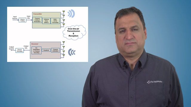
And here you see a block diagram representing an example that is shipping today in Communications Toolbox that simulates that entire link, virtually all on the GPU. So on the transmit side, you've got some CRC, more LDPC encoding because that is typically a long pole in the tent, modulation at both single carrier for QAM and then multi carrier for OFDM, some beamforming-- which is actually very simple, it's just a matrix multiply-- a Rayleigh fading channel, and then undoing on the receive end everything that was done on the transmit end. The link at the bottom shows how you can access that example.

So let's walk through it. Here we are. We're going to accelerate a MIMO-OFDM link simulation using the GPU. Again, I'm not going to run it. My laptop doesn't have a GPU, but I think there are some worthy things to highlight as we walk through this example. So here's our block diagram that we just walked through. Here's the hardware that we happen to use when we published the demo. And really here's the bottom line, if we use CPUs using Parallel Computing Toolbox, 16 workers, we get a factor of 11x speedup, pretty good.

But a single GPU up to a factor of 32x. So this is considerable. But the results are not automatic and I'm going to show you why that is. So here's why. If you have a simulation that has many, many different parallelizable computations, your GPU will give you more benefit. And let me see if I can go ahead and find-- so in this initial case, we've got a relatively short LDPC block length of 648 bits, only two transmit antennas, only four receive antennas. So it's not highly parallelized. I'm going to go on to the end here and cut to the chase.

By the way, here's some path delays and path gains for a multipath channel. Here's where we set up our channel. And then we go ahead and simulate it with a GPU using our tic toc function. Apologies for the scrolling. Now we want to accelerate using parfor and the GPU, but there is a specific spot that I want to get to, to show you the results. Now, for this relatively small parallelized system, the GPU achieved a factor of 3.7x, whereas the 16 workers, once again, they achieved a factor of 11.1x.

So you might ask, well, the CPU is the better solution. In this case, yes, but that's only because the system is not highly parallelized. But we can also create a system that is much more parallelized. And in this case, we've got an LDPC block length of 64,800, very large. And we have 64 transmit antennas and 8 receive antennas, much more parallelized than the previous system. So then lots of setup. And then I just want to cut to the chase once more.

Now the parallel pool of 16 workers accelerates to the tune of 6.7x. The GPU gives you 32x. So once more, the moral of the story is when you have these disparate hardware resources at your disposal, don't automatically assume that one is better than the other, try them both and see which one works better for you. And that is-- let's see. So this is worth showing as well, the BLER curve.

So you see that for the CPU and the GPU, the two curves are spot on. That's because they use the same random number generator seed at the outset. So you're basically running the same numbers through both the CPU and the GPU. The parallel CPU curve is a little bit different because different seeds are being used across each worker in the CPU cluster. The results are statistically valid and believable, but the actual numbers are not identical. And that is about all I would want to say about that example. Let's go back to our slides then.

Our final topic, leveraging FPGAs. So this is really useful when you use FPGA in the loop, or FIL. So if you have a system that has one really, really tall pole, then this FIL technique is probably very, very worthwhile. In this particular block diagram that you see, basically, you have one component that takes up a lot of time, that's an LTE Turbo Decoder. Everything else is more or less housekeeping. So one really tall pole, so FPGA in the loop is very, very useful.

Now be aware, this takes more human investment than either writing better MATLAB code or using PCT with the cores on your laptop, but the gains can be considerable. So using a FIL wizard guides you through the process of generating and then deploying that HDL code onto your FPGA. But look at that last bullet, BER simulation speedups of two orders of magnitude are possible. Again, your mileage may vary, but be thinking if you have one tall pole in your system, then you can put that tall pole on an FPGA and realize many, many gains.

And right here, this is just how you would bring up that wizard at the MATLAB command prompt. Type FIL wizard, and then you would get a GUI that looks much like this. You would have a Simulink model that generates HDL code. And then you would use that generated HDL code with this wizard to create either a MATLAB system object or yet a different Simulink model that can be controlled by MATLAB. And again, you can get many, many x of performance improvement. This will work for both Xilinx, now AMD, and Intel boards.

So let's wrap it all up. You have lots of options to choose from. Probably the easiest thing to try is in the upper left with better MATLAB. The most difficult, but potentially with the biggest benefit is with the FPGAs, with FPGA in the loop. But the point is you can use all of these techniques to accelerate your wireless comms models. Some of these techniques you can use in concert with one another. So if you do really well with the GPU and you do really well with the cloud, imagine what might happen if you use GPUs on the cloud.

But I don't want to leave you without any resources. Take advantage of training. So this graphic here shows MATLAB and Simulink training on how you can accelerate and parallelize your MATLAB code. So these are classes that are available for you. And you don't just have to take my word for it. In a short 30 to 40 minute webinar, you can actually be trained on how to write fast MATLAB code. And with that, I thank you for your attention.