Wavelet Analysis for 3-D Data

Open Live Script

This example shows how to analyze 3-D data using the three-dimensional wavelet analysis tool, and how to display low-pass and high-pass components along a given slice. The example focuses on magnetic resonance images.

A key feature of this analysis is to track the optimal, or at least a good, wavelet-based sparsity of the image which is the lowest percentage of transform coefficients sufficient for diagnostic-quality reconstruction.

To illustrate this, we keep the approximation of a 3-D MRI to show the complexity reduction. The result can be improved if the images were transformed and reconstructed from the largest transform coefficients where the definition of the quality is assessed by medical specialists.

We will see that Wavelet transform for brain images allows efficient and accurate reconstructions involving only 5-10% of the coefficients.

Load and Display 3-D MRI Data

First, load the wmri.mat file which is built from the MRI data set that comes with MATLAB®.

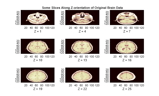
load wmri

We now display some slices along the Z-orientation of the original brain data.

map = pink(90);
idxImages = 1:3:size(X,3);
figure('DefaultAxesXTick',[],'DefaultAxesYTick',[],...
    'DefaultAxesFontSize',8,'Color','w')
colormap(map)
for k = 1:9
    j = idxImages(k);
    subplot(3,3,k)
    image(X(:,:,j))
    xlabel(['Z = ' int2str(j)])
    if k==2
        title('Some Slices Along Z-orientation of Original Brain Data')
    end
end

We now switch to the Y-orientation slice.

perm = [1 3 2];
XP = permute(X,perm);
figure('DefaultAxesXTick',[],'DefaultAxesYTick',[],...
    'DefaultAxesFontSize',8,'Color','w')
colormap(map)
for k = 1:9
    j = idxImages(k);
    subplot(3,3,k)
    image(XP(:,:,j))
    xlabel(['Y = ' int2str(j)])
    if k==2
    	title('Some Slices Along Y-orientation')
    end
end

clear XP

Multilevel 3-D Wavelet Decomposition

Compute the wavelet decomposition of the 3-D data at level 3.

n = 3;                   % Decomposition Level 
w = 'sym4';              % Near Symmetric Wavelet
WT = wavedec3(X,n,w);    % Multilevel 3-D Wavelet Decomposition.

Multilevel 3-D Wavelet Reconstruction

Reconstruct from coefficients the approximations and details for levels 1 to 3.

A = cell(1,n);
D = cell(1,n);
for k = 1:n
    A{k} = waverec3(WT,'a',k);   % Approximations (lowpass components)
    D{k} = waverec3(WT,'d',k);   % Details (highpass components)
end

Check for perfect reconstruction.

err = zeros(1,n);
for k = 1:n
    E = double(X)-A{k}-D{k};
    err(k) = max(abs(E(:)));
end
disp(err)

   1.0e-09 *

    0.3044    0.3044    0.3044

Display Lowpass and Highpass Components

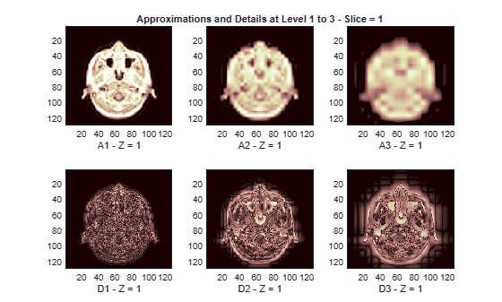
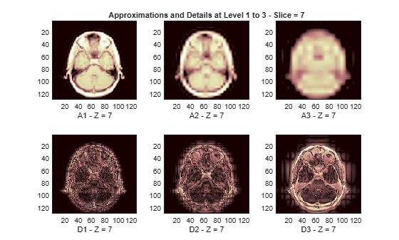
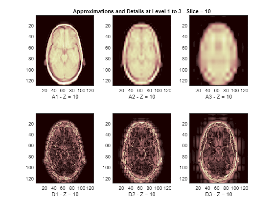
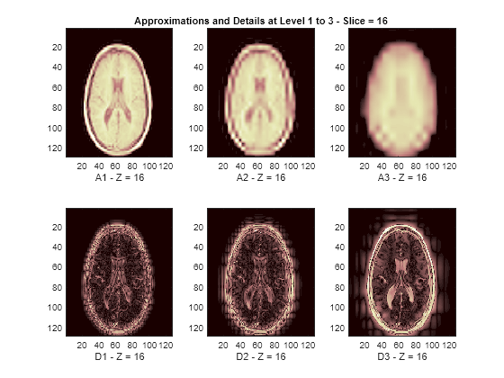
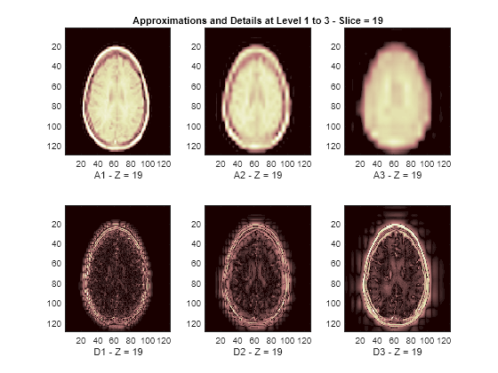
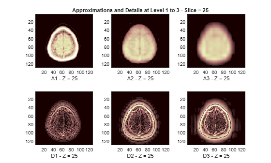
The reconstructed approximations and details along the Z-orientation are displayed below.

nbIMG = 6;
idxImages_New = [1 7 10 16 19 25];
for ik = 1:nbIMG
    j = idxImages_New(ik);
    figure('DefaultAxesXTick',[],'DefaultAxesYTick',[],...
        'DefaultAxesFontSize',8,'Color','w')
    colormap(map)
    for k = 1:n
        labstr = [int2str(k) ' - Z = ' int2str(j)];
        subplot(2,n,k)
        image(A{k}(:,:,j))
        xlabel(['A' labstr])
        if k==2
        	title(['Approximations and Details at Level 1 to 3 - Slice = ' num2str(j)])
        end
        subplot(2,n,k+n)
        imagesc(abs(D{k}(:,:,j)))
        xlabel(['D' labstr])
    end
end

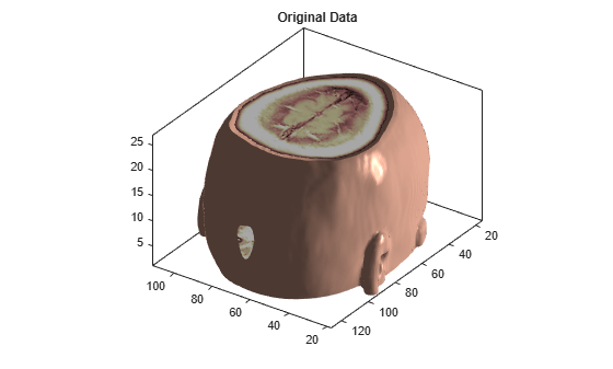
3-D Display of Original Data and Approximation at Level 2

The size of the 3-D original array X is (128 x 128 x 27) = 442368. We can use a 3-D display to show it.

figure('DefaultAxesXTick',[],'DefaultAxesYTick',[],...
        'DefaultAxesFontSize',8,'Color','w')
XR = X;
Ds = smooth3(XR);
hiso = patch(isosurface(Ds,5),'FaceColor',[1,.75,.65],'EdgeColor','none');
hcap = patch(isocaps(XR,5),'FaceColor','interp','EdgeColor','none');
colormap(map)
daspect(gca,[1,1,.4])
lightangle(305,30); 
lighting phong
isonormals(Ds,hiso)
hcap.AmbientStrength = .6;
hiso.SpecularColorReflectance = 0;
hiso.SpecularExponent = 50;
ax = gca;
ax.View = [215,30];
ax.Box = 'On';
axis tight
title('Original Data')

Figure contains an axes object. The axes object with title Original Data contains 2 objects of type patch.

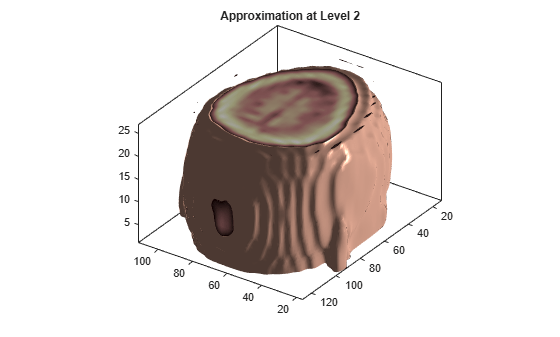
The 3-D array of the coefficients of approximation at level 2, whose size is (22 x 22 x 9) = 4356, is less than 1% the size of the original data. With these coefficients, we can reconstruct A2, the approximation at level 2, which is a kind of compression of the original 3-D array. A2 can also be shown using a 3-D display.

figure('DefaultAxesXTick',[],'DefaultAxesYTick',[],...
        'DefaultAxesFontSize',8,'Color','w')
XR = A{2};
Ds = smooth3(XR);
hiso = patch(isosurface(Ds,5),'FaceColor',[1,.75,.65],'EdgeColor','none');
hcap = patch(isocaps(XR,5),'FaceColor','interp','EdgeColor','none');
colormap(map)
daspect(gca,[1,1,.4])
lightangle(305,30); 
lighting phong
isonormals(Ds,hiso)
hcap.AmbientStrength = .6;
hiso.SpecularColorReflectance = 0;
hiso.SpecularExponent = 50;
ax = gca;
ax.View = [215,30];
ax.Box = 'On';
axis tight
title('Approximation at Level 2')

Figure contains an axes object. The axes object with title Approximation at Level 2 contains 2 objects of type patch.

Summary

This example shows how to use 3-D wavelet functions to analyze 3-D data.