Data Analytics Application with Many MDF-Files

Open Live Script

This example shows you how to investigate vehicle battery power during discharge mode across various drive cycles. The data for this analysis are contained in a set of vehicle log files in MDF format. For this example, we need to build up a mechanism that can "detect" when the vehicle battery is in a given mode. What we are really doing is building a detector to determine when a signal of interest (battery power in this case) meets specific criteria. When the criteria is met, we will call that an "event". Each event will be subsequently "qualified" by imposing time bounds. That is to say an event is "qualified" if it persists for at least 5 seconds (such a qualification step can help limit noise and remove transients). The thresholds shown in this example are illustrative only.

Set Data Source Location

Define the location of the file set to analyze.

dataDir = '*.dat';

Obtain File Set Information

Get the names of all the MDF-files to analyze into a single cell array.

fileList     = dir(dataDir);
fileName     = {fileList(:).name}';
fileDir      = {fileList(:).folder}';
fullFilePath = fullfile(fileDir, fileName)

fullFilePath = 5x1 cell
    {'/tmp/Bdoc23a_2213998_1547508/tpbdc9ff2c/vnt-ex86857001/ADAC.dat' }
    {'/tmp/Bdoc23a_2213998_1547508/tpbdc9ff2c/vnt-ex86857001/ECE.dat'  }
    {'/tmp/Bdoc23a_2213998_1547508/tpbdc9ff2c/vnt-ex86857001/HWFET.dat'}
    {'/tmp/Bdoc23a_2213998_1547508/tpbdc9ff2c/vnt-ex86857001/SC03.dat' }
    {'/tmp/Bdoc23a_2213998_1547508/tpbdc9ff2c/vnt-ex86857001/US06.dat' }

Pre-allocate the Output Data Cell Array

Use a cell array to capture a collection of mini-tables which represent the event data of interest for each individual MDF-file.

numFiles = size(fullFilePath, 1);
eventSet = cell(numFiles, 1)

eventSet=5×1 cell array
    {0x0 double}
    {0x0 double}
    {0x0 double}
    {0x0 double}
    {0x0 double}

Define Event Detection and Channel Information Criteria

chName = 'Power';         % Name of the signal of interest in the MDF-files
thdValue = [5, 55];       % Threshold in KW
thdDuration = seconds(5); % Threshold for event qualification

Loop Through Each MDF-File and Apply the Event Detector Function

eventSet is a cell array which contains a summary table for each file that was analyzed. You can think of this cell array of tables as a set of mini-tables, all with the same format but the contents of each mini-table correspond to the individual MDF-files.

In this example, the event detector not only reports the event start and end times but also some descriptive statistics about the event itself. This kind of aggregation and reporting can be useful for discovery and troubleshooting activities. To understand the MDF-file interfacing and data handling in more detail, open and explore the processMDF function from this example.

Note that the data processing is written such that each MDF-file is parsed atomically and returns into its own index of the resulting cell array. This allows the processing function to leverage parallel computing capability with parfor. parfor and standard for are interchangeable in terms of outputs, but result in varying processing time needed to complete the analysis. To experiment with parallel computing, simply change the for call below to parfor and run this example.

for i = 1:numFiles
    eventSet{i} = processMDF(fullFilePath{i}, chName, thdValue, thdDuration);
end
eventSet{1}

ans=20×8 table
    FileName    EventNumber    EventDuration    EventStart    EventStop     MeanPower_KW    MaxPower_KW    MinPower_KW
    ________    ___________    _____________    __________    __________    ____________    ___________    ___________

    ADAC.dat        2            00:01:22       19.345 sec    101.79 sec       28.456           53.5              5   
    ADAC.dat        3            00:00:08       107.82 sec    116.36 sec       21.295           53.5           5.09   
    ADAC.dat        5            00:00:55        123.8 sec    179.67 sec       28.642           37.2           5.01   
    ADAC.dat        6            00:00:10       189.83 sec    200.36 sec       11.192           54.4            5.1   
    ADAC.dat        8            00:00:40        212.4 sec    252.79 sec       28.539           37.4           5.01   
    ADAC.dat        9            00:00:08       258.76 sec    267.37 sec       21.289           53.7           5.02   
    ADAC.dat        11           00:00:44       274.81 sec    319.79 sec       28.554           37.2           5.08   
    ADAC.dat        12           00:00:08       325.75 sec    334.37 sec       21.279           53.7           5.05   
    ADAC.dat        14           00:00:44       341.81 sec    386.79 sec       28.554           37.2           5.08   
    ADAC.dat        15           00:00:08       392.75 sec    401.37 sec       21.278           53.7           5.04   
    ADAC.dat        17           00:00:44       408.81 sec    453.67 sec       28.579           37.2           5.08   
    ADAC.dat        18           00:00:07       463.77 sec    471.37 sec       11.895         54.676           5.04   
    ADAC.dat        20           00:00:40       483.44 sec    523.79 sec       28.544         37.363         5.0682   
    ADAC.dat        21           00:00:08       529.75 sec    538.37 sec       21.279           53.7           5.05   
    ADAC.dat        23           00:00:44       545.81 sec    590.79 sec       28.553           37.2           5.08   
    ADAC.dat        24           00:00:08       596.75 sec    605.37 sec       21.279           53.7           5.05   
      ⋮

Concatenate Results

Combine the contents of the cell array eventSet into a single table. We can now use the table eventSummary for subsequent analysis. The head function is used to display the first 5 rows of the table eventSummary.

eventSummary = vertcat(eventSet{:});
disp(head(eventSummary, 5))

    FileName    EventNumber    EventDuration    EventStart    EventStop     MeanPower_KW    MaxPower_KW    MinPower_KW
    ________    ___________    _____________    __________    __________    ____________    ___________    ___________

    ADAC.dat         2           00:01:22       19.345 sec    101.79 sec       28.456          53.5              5    
    ADAC.dat         3           00:00:08       107.82 sec    116.36 sec       21.295          53.5           5.09    
    ADAC.dat         5           00:00:55        123.8 sec    179.67 sec       28.642          37.2           5.01    
    ADAC.dat         6           00:00:10       189.83 sec    200.36 sec       11.192          54.4            5.1    
    ADAC.dat         8           00:00:40        212.4 sec    252.79 sec       28.539          37.4           5.01

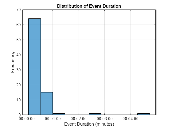
Visualize Summary Results to Determine Next Steps

Look at an overview of the event durations.

histogram(eventSummary.EventDuration)
grid on
title 'Distribution of Event Duration'
xlabel 'Event Duration (minutes)'
ylabel 'Frequency'

Figure contains an axes object. The axes object with title Distribution of Event Duration, xlabel Event Duration (minutes), ylabel Frequency contains an object of type histogram.

Now look at Mean Power vs. Event Duration.

scatter(eventSummary.MeanPower_KW, minutes(eventSummary.EventDuration))
grid on
xlabel 'MeanPower(KW)'
ylabel 'Event Duration (minutes)'
title 'Mean Power vs. Event Duration'

Figure contains an axes object. The axes object with title Mean Power vs. Event Duration, xlabel MeanPower(KW), ylabel Event Duration (minutes) contains an object of type scatter.

Deep Dive an Event of Interest

Inspect the event that lasted for more than 4 minutes. First, create a mask to find the case of interest. msk is a logical index that shows which rows of the table eventSummary meet the specified criteria.

msk = eventSummary.EventDuration > minutes(4);

Pull out the rows of the table eventSummary that meet the criteria specified and display the results.

eventOfInterest = eventSummary(msk, :);
disp(eventOfInterest)

    FileName     EventNumber    EventDuration    EventStart    EventStop     MeanPower_KW    MaxPower_KW    MinPower_KW
    _________    ___________    _____________    __________    __________    ____________    ___________    ___________

    HWFET.dat        18           00:04:43       297.22 sec    580.37 sec       12.275          30.2          5.0024

Visualize This Event in the Context of the Entire Drive Cycle

We need the full file path and file name to read the data from the MDF-file. The table eventOfInterest has the filename because we kept track of that. It does not have the full file path to that file. To get this information we will apply a bit of set theory to our original list of filenames and paths. First, find the full file path of the file of interest.

fileMsk = find(ismember(fileName, eventOfInterest.FileName))

fileMsk = 3

Read the channel data of interest from the MDF-file using mdfRead.

data = mdfRead(fullFilePath{fileMsk}, Channel=chName)

data = 1x1 cell array
    {79176x1 timetable}

data{1}

ans=79176×1 timetable
        time           Power  
    _____________    _________

    0.0048987 sec            0
    0.0088729 sec            0
    0.01 sec                 0
    0.013223 sec             0
    0.016446 sec             0
    0.019668 sec             0
    0.02 sec                 0
    0.021658 sec      -2.4e-28
    0.023878 sec     -3.42e-15
    0.026098 sec     -1.04e-14
    0.027766 sec      -1.9e-14
    0.029433 sec     -3.14e-14
    0.03 sec         -3.66e-14
    0.031341 sec     -5.14e-14
    0.032681 sec     -6.92e-13
    0.034022 sec     -1.56e-12
      ⋮

Visualize Using a Custom Plotting Function

Custom plotting functions are useful for encapsulation and reuse. Visualize the event in the context of the entire drive cycle. To understand how the visualization was created, open and explore the eventPlotter function from this example.

eventPlotter(data{1}, eventOfInterest)

Figure contains an axes object. The axes object with title HWFET.dat, xlabel Time (min), ylabel Power (KW) contains 2 objects of type line. One or more of the lines displays its values using only markers These objects represent Raw Signal, Event.