Compute Optical Flow Velocities
This example shows how to compute the optical flow velocities for a moving object in a video or image sequence.
Read two image frames from an image sequence into the MATLAB® workspace.
I1 = imread('car_frame1.png');
I2 = imread('car_frame2.png');
Open the Simulink® model.
modelname = 'ex_blkopticalflow.slx';
open_system(modelname)
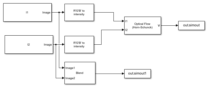
The model reads the images by using the Image From Workspace block. To compute the optical flow velocities, you must first convert the input color images to intensity images by using the Color Space Conversion block. Then, find the velocities by using the Optical Flow block with these parameter values:
Method -
Horn-SchunckCompute optical flow between -
Two imagesSmoothness factor -
1Stop iterative solution -
When maximum number of iterations is reachedMaximum number of iterations -
10Velocity output -
Horizontal and vertical components in complex form
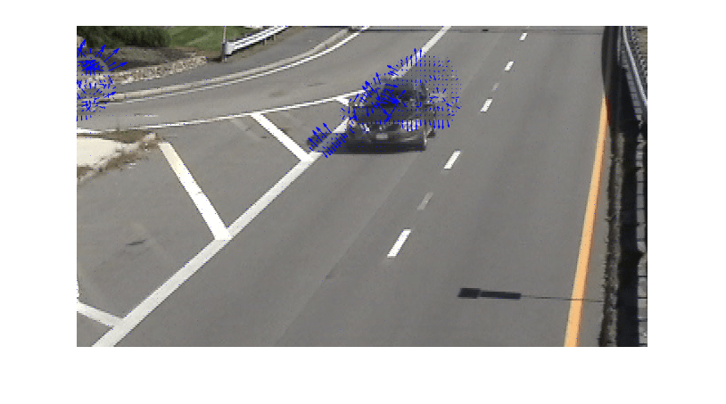
Overlay both the image frames by using the Compositing block and use the overlaid image to plot the results.
Run the model.
out = sim(modelname);
Read the output velocities and the overlaid image.
Vx = real(out.simout);
Vy = imag(out.simout);
img = out.simout1;
Create an optical flow object by using the opticalFlow function.
flow = opticalFlow(Vx,Vy);
Display the overlaid image and plot the velocity vectors by using the plot function.
figure
imshow(img)
hold on
plot(flow,'DecimationFactor',[5 5],'ScaleFactor',40)