Functional Derivatives Tutorial
This example shows how to use functional derivatives in the Symbolic Math Toolbox™ using the example of the wave equation. This example performs calculations symbolically to obtain analytic results. The wave equation for a string fixed at its ends is solved using functional derivatives. A functional derivative is the derivative of a functional with respect to the function that the functional depends on. The Symbolic Math Toolbox implements functional derivatives using the functionalDerivative function.
Solving the wave equation is one application of functional derivatives. It describes the motion of waves, from the motion of a string to the propagation of an electromagnetic wave, and is an important equation in physics. You can apply the techniques illustrated in this example to applications in the calculus of variations from solving the Brachistochrone problem to finding minimal surfaces of soap bubbles.
Consider a string of length L suspended between the two points x = 0 and x = L. The string has a characteristic density per unit length and a characteristic tension. Define the length, mass density, and tension as constants for later use. For simplicity, set these constants to 1.
Length = 1;
Density = 1;
Tension = 1;
If the string is in motion, the string's kinetic and potential energy densities are a function of its displacement from rest S(x,t), which varies with position x and time t. If d is the mass density per unit length, the kinetic energy density is
The potential energy density is
where r is the tension.
Enter these equations in MATLAB®. Since length must be positive, set this assumption. This assumption allows simplify to simplify the resulting equations into the expected form.
syms S(x,t) d r v L
assume(L>0)
T(x,t) = d/2*diff(S,t)^2;
V(x,t) = r/2*diff(S,x)^2;
The action density A is T-V. The Principle of Least Action states that action is always minimized. Determine the condition for minimum action by finding the functional derivative of A with respect to S using functionalDerivative and equate it to zero.
A = T-V;
eqn = functionalDerivative(A,S) == 0
eqn(x, t) =
Simplify the equation using simplify. Convert the equation into its expected form by substituting for r/d with the square of the wave velocity v.
eqn = simplify(eqn)/r;
eqn = subs(eqn,r/d,v^2)
eqn(x, t) =
Solve the equation using the method of separation of variables. Set S(x,t) = U(x)*V(t) to separate the dependence on position x and time t. Separate both sides of the resulting equation using children.
syms U(x) V(t)
eqn2 = subs(eqn,S(x,t),U(x)*V(t));
eqn2 = eqn2/(U(x)*V(t))
eqn2(x, t) =
tmp = children(eqn2);
Both sides of the equation depend on different variables, yet are equal. This is only possible if each side is a constant. Equate each side to an arbitrary constant C to get two differential equations.
syms C
eqn3 = tmp(1) == C
eqn3 =
eqn4 = tmp(2) == C
eqn4 =
Solve the differential equations using dsolve with the condition that displacement is 0 at x = 0 and t = 0. Simplify the equations to their expected form using simplify with the Steps option set to 50.
V(t) = dsolve(eqn3,V(0)==0,t);
U(x) = dsolve(eqn4,U(0)==0,x);
V(t) = simplify(V(t),'Steps',50)
V(t) =
U(x) = simplify(U(x),'Steps',50)U(x) =
Obtain the constants in the equations.
p1 = setdiff(symvar(U(x)),sym([C,x]))
p1 =
p2 = setdiff(symvar(V(t)),sym([C,v,t]))
p2 =
The string is fixed at the positions x = 0 and x = L. The condition U(0) = 0 already exists. Apply the boundary condition that U(L) = 0 and solve for C.
eqn_bc = U(L) == 0;
[solC,param,cond] = solve(eqn_bc,C,'ReturnConditions',true)
solC =
param =
cond =
assume(cond)
The solution S(x,t) is the product of U(x) and V(t). Find the solution, and substitute the characteristic values of the string into the solution to obtain the final form of the solution.
S(x,t) = U(x)*V(t);
S = subs(S,C,solC);
S = subs(S,[L v],[Length sqrt(Tension/Density)]);
The parameters p1 and p2 determine the amplitude of the vibrations. Set p1 and p2 to 1 for simplicity.
S = subs(S,[p1 p2],[1 1]);
S = simplify(S,'Steps',50)
S(x, t) =
The string has different modes of vibration for different values of k. Plot the first four modes for an arbitrary value of time t. Use the param argument returned by solve to address parameter k.
Splot(x) = S(x,0.3);
figure(1)
hold on
grid on
ymin = double(coeffs(Splot));
for i = 1:4
    yplot = subs(Splot,param,i);
    fplot(yplot,[0 Length])
end
ylim([-ymin ymin])
legend('k = 1','k = 2','k = 3','k = 4','Location','best')
xlabel('Position (x)')
ylabel('Displacement (S)')
title('Modes of a string')

The wave equation is linear. This means that any linear combination of the allowed modes is a valid solution to the wave equation. Hence, the full solution to the wave equation with the given boundary conditions and initial values is a sum over allowed modes
where denotes arbitrary constants.
Use symsum to sum the first five modes of the string. On a new figure, display the resulting waveform at the same instant of time as the previous waveforms for comparison.
figure(2)
S5(x) = 1/5*symsum(S,param,1,5);
fplot(subs(S5,t,0.3),[0 Length])
ylim([-ymin ymin])
grid on
xlabel('Position (x)')
ylabel('Displacement (S)')
title('Summation of first 5 modes')
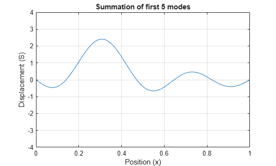
The figure shows that summing modes allows you to model a qualitatively different waveform. Here, we specified the initial condition is for all .
You can calculate the values in the equation by specifying a condition for initial velocity
The appropriate summation of modes can represent any waveform, which is the same as using the Fourier series to represent the string's motion.