Find Extremum of Multivariate Function and Its Approximation
This example shows how to find the extremum of a multivariate function and its approximation near the extremum point. This example uses symbolic matrix variables to represent the multivariate function and its derivatives. Symbolic matrix variables are available starting in R2021a.
Consider the multivariate function , where is a 2-by-1 vector and is a 2-by-2 matrix. To find a local extremum of this function, compute a root of the derivative of . In other words, find the solution of the derivative .
Create Function and Find Its Derivative
Create the vector and the matrix as symbolic matrix variables. Define the function .
syms x [2 1] matrix
syms A [2 2] matrix
f = sin(x.'*A*x)
f =
Compute the derivative D of the function with respect to the vector . The derivative D is displayed in compact matrix notation in terms of and .
D = diff(f,x)
D =
Convert symmatrix Objects to sym Objects
The symbolic matrix variables x, A, f, and D are symmatrix objects. These objects represent matrices, vectors, and scalars in compact matrix notation. To show the components of these variables, convert the symmatrix objects to sym objects using symmatrix2sym.
xsym = symmatrix2sym(x)
xsym =
Asym = symmatrix2sym(A)
Asym =
fsym = symmatrix2sym(f)
fsym =
Dsym = symmatrix2sym(D)
Dsym =
Substitute Numeric Values and Find the Minimum
Suppose you are interested in the case where the value of is [2 -1; 0 3]. Substitute this value into the function fsym.
fsym = subs(fsym,Asym,[2 -1; 0 3])
fsym =
Substitute the value of into the derivative Dsym
Dsym = subs(Dsym,Asym,[2 -1; 0 3])
Dsym =
Then, apply the symbolic function solve to get a root of the derivative.
[xmin,ymin] = solve(Dsym,xsym,'PrincipalValue',true);
x0 = [xmin; ymin]
x0 =
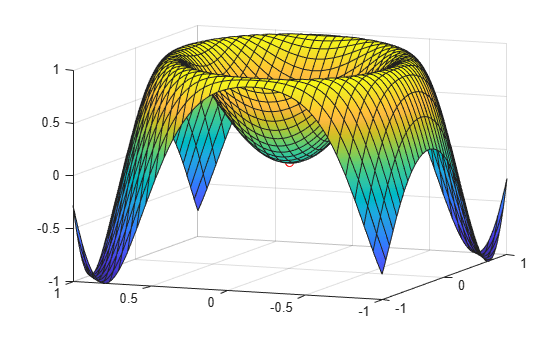
Plot the function together with the extremum solution . Set the plot interval to and as the second argument of fsurf. Use fplot3 to plot the coordinates of the extremum solution.
fsurf(fsym,[-1 1 -1 1])
hold on
fplot3(xmin,ymin,subs(fsym,xsym,x0),'ro')
view([-68 13])
Approximate Function Near Its Minimum
You can approximate a multivariate function around a point with a multinomial using the Taylor expansion.
Here, the term is the gradient vector, and is the Hessian matrix of the multivariate function calculated at .
Find the Hessian matrix and return the result as a symbolic matrix variable.
H = diff(f,x,x.')
H =
Convert the Hessian matrix to the sym data type, which represents the matrix in its component form. Use subs to evaluate the Hessian matrix for = [2 -1; 0 3] at the minimum point .
Hsym = symmatrix2sym(H);
Hsym = subs(Hsym,Asym,[2 -1; 0 3]);
H0 = subs(Hsym,xsym,x0)
H0 =
Evaluate the gradient vector at .
D0 = subs(Dsym,xsym,x0)
D0 =
Compute the Taylor approximation to the function near its minimum.
fapprox = subs(fsym,xsym,x0) + D0*(xsym-x0) + 1/2*(xsym-x0).'*H0*(xsym-x0)
fapprox =
Plot the function approximation on the same graph that shows and .
hold on
fsurf(fapprox,[-1 1 -1 1])
zlim([-1 3])