Differentiation
This example shows how to analytically find and evaluate derivatives using Symbolic Math Toolbox™. In the example you will find the 1st and 2nd derivative of f(x) and use these derivatives to find local maxima, minima and inflection points.
Find Local Minima and Maxima Using First Derivatives
Computing the first derivative of an expression helps you find local minima and maxima of that expression. Before creating a symbolic expression, create symbolic variables.
syms xBy default, solutions that include imaginary components are included in the results. Here, consider only real values of x by setting the assumption that x is real.
assume(x,"real")As an example, create a rational expression (such as a fraction where the numerator and denominator are polynomial expressions).
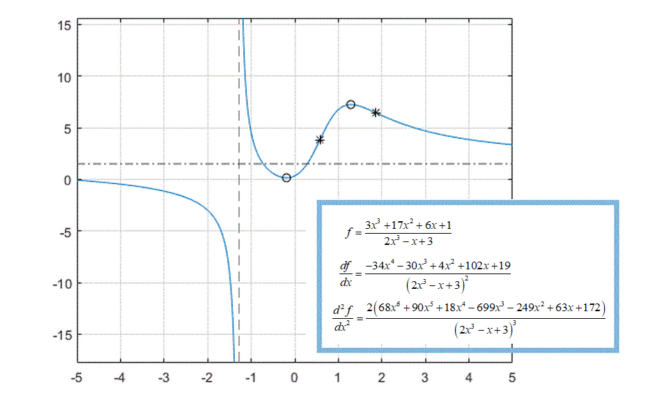
f = (3*x^3 + 17*x^2 + 6*x + 1)/(2*x^3 - x + 3)
f =
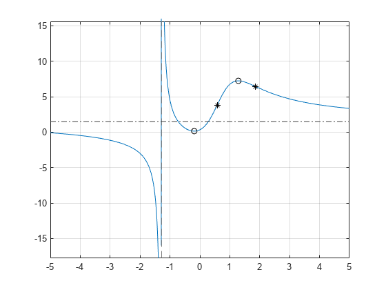
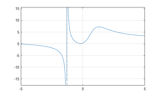
Plotting this expression shows that the expression has horizontal and vertical asymptotes, a local minimum between –1 and 0, and a local maximum between 1 and 2.
fplot(f)
grid
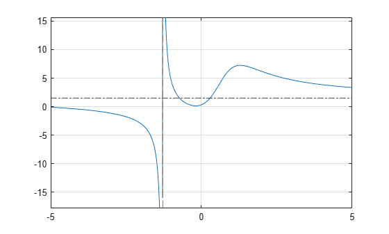
To find the horizontal asymptote, compute the limits of f for x approaching positive and negative infinities. The horizontal asymptote is y = 3/2.
lim_left = limit(f,x,-Inf)
lim_left =
lim_right = limit(f,x,Inf)
lim_right =
Add this horizontal asymptote to the plot.
hold on
plot(xlim,[lim_right lim_right],LineStyle="-.",Color=[0.25 0.25 0.25])
To find the vertical asymptote of f, find the poles of f.
pole_pos = poles(f,x)
pole_pos =
Approximate the exact solution numerically by using the double function.
double(pole_pos)
ans =
-1.2896
Now find the local minimum and maximum of f. If a point is a local extremum (either minimum or maximum), the first derivative of the expression at that point is equal to zero. Compute the derivative of f using diff.
g = diff(f,x)
g =
To find the local extrema of f, solve the equation g == 0.
g0 = solve(g,x)
g0 =
Approximate the exact solution numerically by using the double function.
double(g0)
ans = 2×1

   -0.1892
    1.2860
The expression f has a local maximum at x = 1.286 and a local minimum at x = -0.189. Obtain the function values at these points using subs.
f0 = subs(f,x,g0)
f0 =
Approximate the exact solution numerically by using the double function on the variable f0.
double(f0)
ans = 2×1

    0.1427
    7.2410
Add point markers to the graph at the extrema.
plot(g0,f0,"ok")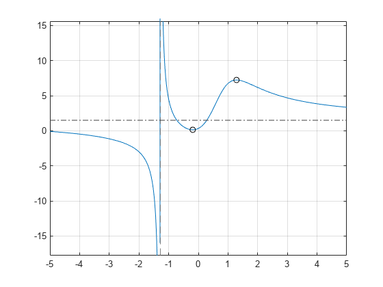
Find Inflection Points Using Second Derivatives
Computing the second derivative lets you find inflection points of the expression. The most efficient way to compute second or higher-order derivatives is to use the parameter that specifies the order of the derivative.
h = diff(f,x,2)
h =
Now simplify that result.
h = simplify(h)
h =
To find inflection points of f, solve the equation h = 0. Here, use the numeric solver vpasolve to calculate floating-point approximations of the solutions.
h0 = vpasolve(h,x)
h0 =
The expression f has two inflection points: x = 1.865 and x = 0.579. Note that vpasolve also returns complex solutions. Exclude the complex solutions.
h0(imag(h0)~=0) = []
h0 =
Add markers to the plot showing the inflection points:
plot(h0,subs(f,x,h0),"*k")
hold off