Solve Difference Equations Using Z-Transform
Solve difference equations by using Z-transforms in Symbolic Math Toolbox™ with this workflow. For simple examples on the Z-transform, see ztrans and iztrans.
Definition: Z-transform
The Z-transform of a function f(n) is defined as
Concept: Using Symbolic Workflows
Symbolic workflows keep calculations in the natural symbolic form instead of numeric form. This approach helps you understand the properties of your solution and use exact symbolic values. You substitute numbers in place of symbolic variables only when you require a numeric result or you cannot continue symbolically. For details, see Choose Numeric or Symbolic Arithmetic. Typically, the steps are:
Declare equations.
Solve equations.
Substitute values.
Plot results.
Analyze results.
Workflow: Solve "Rabbit Growth" Problem Using Z-Transform
Declare Equations
You can use the Z-transform to solve difference equations, such as the well-known "Rabbit Growth" problem. If a pair of rabbits matures in one year, and then produces another pair of rabbits every year, the rabbit population at year is described by this difference equation.
Declare the equation as an expression assuming the right side is 0. Because n represents years, assume that n is a positive integer. This assumption simplifies the results.
syms p(n) z
assume(n>=0 & in(n,"integer"))
f = p(n+2) - p(n+1) - p(n)
f =
Solve Equations
Find the Z-transform of the equation.
fZT = ztrans(f,n,z)
fZT =
The function solve solves only for symbolic variables. Therefore, to use solve, first substitute ztrans(p(n),n,z) with the variables pZT.
syms pZT
fZT = subs(fZT,ztrans(p(n),n,z),pZT)
fZT =
Solve for pZT.
pZT = solve(fZT,pZT)
pZT =
Calculate by computing the inverse Z-transform of pZT. Simplify the result.
pSol = iztrans(pZT,z,n);
pSol = simplify(pSol)
pSol =
Substitute Values
To plot the result, first substitute the values of the initial conditions. Let p(0) and p(1) be 1 and 2, respectively.
pSol = subs(pSol,[p(0) p(1)],[1 2])
pSol =
Plot Results
Show the growth in rabbit population over time by plotting pSol.
nValues = 1:10;
pSolValues = subs(pSol,n,nValues);
pSolValues = double(pSolValues);
pSolValues = real(pSolValues);
stem(nValues,pSolValues)
title("Rabbit Population")
xlabel("Years (n)")
ylabel("Population p(n)")
grid on

Analyze Results
The plot shows that the solution appears to increase exponentially. However, because the solution pSol contains many terms, finding the terms that produce this behavior requires analysis.
Because all the functions in pSol can be expressed in terms of exp, rewrite pSol to exp. Simplify the result by using simplify with 80 additional simplification steps. Now, you can analyze pSol.
pSol = rewrite(pSol,"exp");
pSol = simplify(pSol,"Steps",80)
pSol =
Visually inspect pSol. Notice that pSol is a sum of terms. Each term is a ratio that can increase or decrease as n increases. For each term, you can confirm this hypothesis in several ways:
Check if the limit at
n = Infgoes to0orInfby usinglimit.Plot the term for increasing
nand check behavior.Calculate the value at a large value of
n.
For simplicity, use the third approach. Calculate the terms at n = 100, and then verify the approach. First, find the individual terms by using children, substitute for n, and convert to double.
pSolTerms = children(pSol);
pSolTerms = [pSolTerms{:}];
pSolTermsDbl = subs(pSolTerms,n,100);
pSolTermsDbl = double(pSolTermsDbl)
pSolTermsDbl = 1×4
1021 ×
1.5841 0.0000 -0.6568 -0.0000
The result shows that some terms are 0 while other terms have a large magnitude. Hypothesize that the large-magnitude terms produce the exponential behavior. Approximate pSol with these terms.
idx = abs(pSolTermsDbl)>1; % use arbitrary cutoff
pApprox = pSolTerms(idx);
pApprox = sum(pApprox)
pApprox =
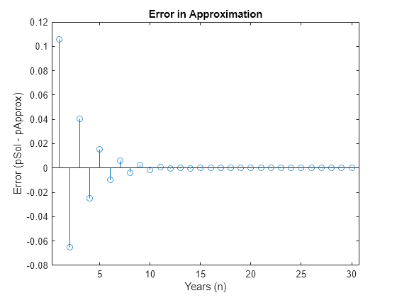
Verify the hypothesis by plotting the approximation error between pSol and pApprox. As expected, the error goes to 0 as n increases. This result demonstrates how symbolic calculations help you analyze your problem.
Perror = pSol - pApprox;
nValues = 1:30;
Perror = subs(Perror,n,nValues);
stem(nValues,Perror)
xlabel("Years (n)")
ylabel("Error (pSol - pApprox)")
title("Error in Approximation")
References
[1] Andrews, L.C., Shivamoggi, B.K., Integral Transforms for Engineers and Applied Mathematicians, Macmillan Publishing Company, New York, 1986
[2] Crandall, R.E., Projects in Scientific Computation, Springer-Verlag Publishers, New York, 1994
[3] Strang, G., Introduction to Applied Mathematics, Wellesley-Cambridge Press, Wellesley, MA, 1986