Fourier and Inverse Fourier Transforms
This page shows the workflow for Fourier and inverse Fourier transforms in Symbolic Math Toolbox™. For simple examples, see fourier and ifourier. Here, the workflow for Fourier
transforms is demonstrated by calculating the deflection of a beam due to a force. The
associated differential equation is solved by the Fourier transform.
Fourier Transform Definition
The Fourier transform of f(x) with respect to x at w is
The inverse Fourier transform is
Concept: Using Symbolic Workflows
Symbolic workflows keep calculations in the natural symbolic form instead of numeric form. This approach helps you understand the properties of your solution and use exact symbolic values. You substitute numbers in place of symbolic variables only when you require a numeric result or you cannot continue symbolically. For details, see Choose Numeric or Symbolic Arithmetic. Typically, the steps are:
Declare equations.
Solve equations.
Substitute values.
Plot results.
Analyze results.
Calculate Beam Deflection Using Fourier Transform
Define Equations
Fourier transform can be used to solve ordinary and partial differential equations. For example, you can model the deflection of an infinitely long beam resting on an elastic foundation under a point force. A corresponding real-world example is railway tracks on a foundation. The railway tracks are the infinitely long beam while the foundation is elastic.
Let
E be the elasticity of the beam (or railway track).
I be the second moment of area of the cross-section of the beam.
k be the spring stiffness of the foundation.
The differential equation is
Define the function y(x) and the variables. Assume
E, I, and k are positive.
syms Y(x) w E I k f
assume([E I k] > 0)
Assign units to the variables by using symunit.
u = symunit;
Eu = E*u.Pa;    % Pascal
Iu = I*u.m^4;   % meter^4
ku = k*u.N/u.m^2;  % Newton/meter^2
X = x*u.m;
F = f*u.N/u.m;
Define the differential equation.
eqn = diff(Y,X,4) + ku/(Eu*Iu)*Y == F/(Eu*Iu)
eqn(x) =
diff(Y(x), x, x, x, x)*(1/[m]^4) + ((k*Y(x))/(E*I))*([N]/([Pa]*[m]^6)) == ...
        (f/(E*I))*([N]/([Pa]*[m]^5))
Represent the force f by the Dirac delta function δ(x).
eqn = subs(eqn,f,dirac(x))
eqn(x) =
diff(Y(x), x, x, x, x)*(1/[m]^4) + ((k*Y(x))/(E*I))*([N]/([Pa]*[m]^6)) == ...
        (dirac(x)/(E*I))*([N]/([Pa]*[m]^5))
Solve Equations
Calculate the Fourier transform of eqn by using
fourier on both sides of eqn. The Fourier
transform converts differentiation into exponents of w.
eqnFT = fourier(lhs(eqn)) == fourier(rhs(eqn))
eqnFT =
w^4*fourier(Y(x), x, w)*(1/[m]^4) + ((k*fourier(Y(x), x, w))/(E*I))*([N]/([Pa]*[m]^6)) ...
        == (1/(E*I))*([N]/([Pa]*[m]^5))
Isolate fourier(Y(x),x,w) in the equation.
eqnFT = isolate(eqnFT, fourier(Y(x),x,w))
eqnFT =
fourier(Y(x), x, w) == (1/(E*I*w^4*[Pa]*[m]^2 + k*[N]))*[N]*[m]
Calculate Y(x) by calculating the inverse Fourier transform of the
right side. Simplify the result.
YSol = ifourier(rhs(eqnFT));
YSol = simplify(YSol)
YSol =
((exp(-(2^(1/2)*k^(1/4)*abs(x))/(2*E^(1/4)*I^(1/4)))*sin((2*2^(1/2)*k^(1/4)*abs(x) + ...
        pi*E^(1/4)*I^(1/4))/(4*E^(1/4)*I^(1/4))))/(2*E^(1/4)*I^(1/4)*k^(3/4)))*[m]
Check that YSol has the correct dimensions by substituting
YSol into eqn and using the
checkUnits function. checkUnits returns logical
1 (true), meaning eqn now has
compatible units of the same physical dimensions.
checkUnits(subs(eqn,Y,YSol))
ans =
  struct with fields:

    Consistent: 1
    Compatible: 1
Separate the expression from the units by using
separateUnits.
YSol = separateUnits(YSol)
YSol =
(exp(-(2^(1/2)*k^(1/4)*abs(x))/(2*E^(1/4)*I^(1/4)))*sin((2*2^(1/2)*k^(1/4)*abs(x) + ...
        pi*E^(1/4)*I^(1/4))/(4*E^(1/4)*I^(1/4))))/(2*E^(1/4)*I^(1/4)*k^(3/4))
Substitute Values
Use the values E = 106 Pa, I = 10-3
m4, and k = 106
N/m2. Substitute these values into YSol and convert to
floating point by using vpa with 16 digits of accuracy.
values = [1e6 1e-3 1e5];
YSol = subs(YSol,[E I k],values);
YSol = vpa(YSol,16)
YSol =
0.0000158113883008419*exp(-2.23606797749979*abs(x))*sin(2.23606797749979*abs(x) + ...
        0.7853981633974483)
Plot Results
Plot the result by using fplot.
fplot(YSol)
xlabel('x')
ylabel('Deflection y(x)')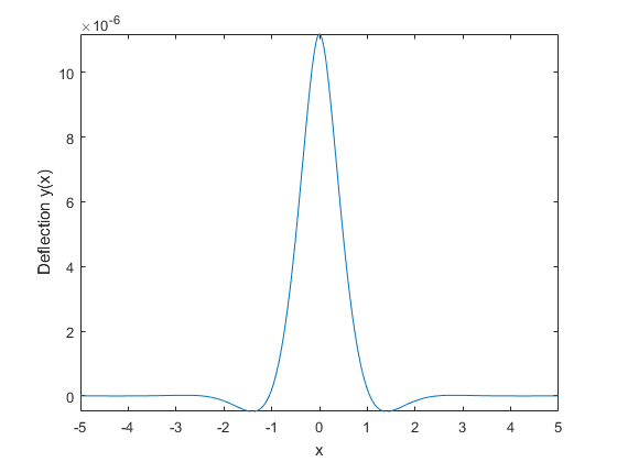
Analyze Results
The plot shows that the deflection of a beam due to a point force is highly localized. The deflection is greatest at the point of impact and then decreases quickly. The symbolic result enables you to analyze the properties of the result, which is not possible with numeric results.
Notice that YSol is a product of terms. The term with
sin shows that the response is vibrating oscillatory behavior. The
term with exp shows that the oscillatory behavior is quickly damped by
the exponential decay as the distance from the point of impact increases.