mhsample

Generate Markov chain sample using Metropolis–Hastings sampler

Syntax

sample = mhsample(start,numsamples,Name=Value)

[sample,acceptance] = mhsample(___)

Description

sample = mhsample(start,numsamples,Name=Value) returns a sequence (Markov chain) of numsamples random draws from the target stationary distribution by using the Metropolis–Hastings sampler, a Markov chain Monte Carlo (MCMC) algorithm. mhsample initializes the sampler from start, and then draws samples using the proposal random number generator.

You must specify these inputs using name-value arguments:

• Target PDF Form — Specify the target stationary distribution or its log by using PDF or LogPDF, respectively.

• Proposal Random Number Generator — Specify a supported distribution name or function by using Proposal or PropRND, respectively.

• Proposal Distribution Description — When you use Proposal, specify the proposal scale using Scale. When you use PropRND, specify one of the following:

  • Symmetric to indicate whether the proposal distribution is symmetric

  • PropPDF to specify the proposal probability distribution function (pdf)

  • LogPropPDF to specify the log of the proposal pdf

You can specify additional options by setting more name-value arguments. For example, BurnIn=100,Thin=4 removes the first 100 draws from the raw generated Markov chain (burn-in period of 100), retains every fourth draw of the remaining chain (thinning factor of 4), and then returns the resulting processed chain in sample.

For details on which Metropolis–Hastings sampler algorithm mhsample implements, see Algorithms.

[sample,acceptance] = mhsample(___) also returns the acceptance rate acceptance of proposal draws for each Markov chain. When computing acceptance, mhsample includes any samples omitted for the specified thinning factor and burn-in period.

Examples

Estimate Second Moment of Gamma Distribution Using Random-Walk Metropolis–Hastings Sampler with Gaussian Proposal

Consider sampling from the Gamma(2.43,1) distribution, and then estimating its second moment.

Create a function that computes the pdf of the Gamma(2.43,1) distribution for an input value.

alpha = 2.43;
beta = 1;
targetPDF = @(x)gampdf(x,alpha,beta);

Although this example uses the exact pdf, typically the target pdf is known only up to a proportionality constant.

Draw 5000 samples (a length 5000 Markov chain) from the Gamma(2.43,1) distribution using the Random-Walk Metropolis–Hastings sampler with a Gaussian proposal and standard deviation of 10. Initialize the sampler from a random positive value in (0,1).

rng(1,"twister")  % For reproducibility
numsamples = 5000;
start = rand(1);
sample = mhsample(start,numsamples,PDF=targetPDF,Proposal="gaussian", ...
    Scale=10);

Create a time series plot of the Markov chain.

figure
plot(sample)
title("Random-Walk Metropolis-Hastings Sample from Gamma(2.43,1)")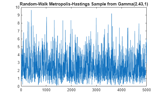

The plot shows little transient behavior and almost no serial correlation, indicating that the Markov chain mixes well.

Fit a Gamma distribution to the sample.

fitdist(sample,"gamma")

ans = 
  GammaDistribution

  Gamma distribution
    a =  2.65537   [2.55891, 2.75547]
    b = 0.921943   [0.885152, 0.960264]

The parameter estimates are close to the true values.

Visually assess the fit.

histfit(sample,15,"gamma")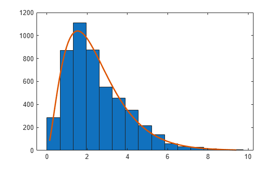

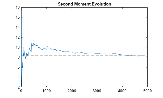
Estimate the second moment of a Gamma distribution by using the sample to perform numerical integration. Compare the result to the theoretical second moment.

x2hat = sum(sample.^2)/numsamples

x2hat = 
8.2449

truex2 = beta^2*gamma(alpha+2)/gamma(alpha)

truex2 = 
8.3349

The estimate is close to the theoretical value.

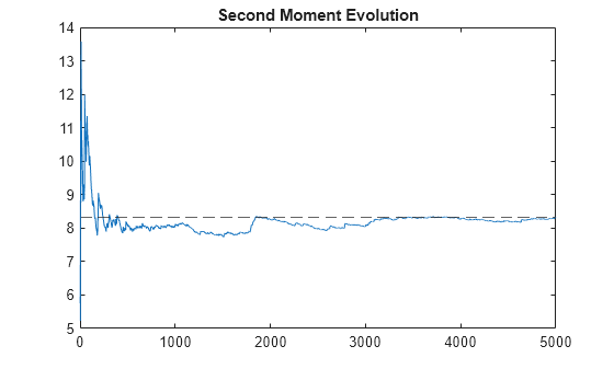
Explore the convergence rate of the estimate by plotting its evolution.

figure
x2hatchain = cumsum(sample.^2)./(1:numsamples)';
plot(x2hatchain)
hold on
yline(truex2,"--")
title("Second Moment Evolution")

Estimate Second Moment of Gamma Distribution Using Independent Metropolis–Hastings Sampler with Custom Proposal

Consider sampling from the Gamma(2.43,1) distribution, and then estimating its second moment. This example uses a custom proposal and the Independent Metropolis–Hastings sampler algorithm. In this case, you must use the default value of Symmetric (false) and specify the proposal distribution pdf (either PropPDF or LogPropPDF).

Create a function that computes the pdf of the Gamma(2.43,1) distribution for an input value.

alpha = 2.43;
beta = 1;
targetPDF = @(x)gampdf(x,alpha,beta);

Although this example uses the exact pdf, typically the target pdf is known only up to a proportionality constant.

The sum of $\mathit{n}$ exponential random variables with rate ${\beta }^{-1}$ has a gamma distribution with shape $\mathit{n}$ and scale $\beta$.

Create a function that accepts the current state of the chain xt, draws $\lfloor \alpha \rfloor$ random values from an exponential distribution with rate ${\beta }^{-1}$, and then sums the results. This function is the proposal random number generator.

n = floor(alpha);
propRND = @(xt)sum(exprnd(1/beta,n,1));

Create a function that accepts the proposal draw y and current state of the chain xt, and computes the pdf of the proposed draw, which is Gamma($\lfloor \alpha \rfloor$,$\beta$). The proposal pdf is independent of the current state of the Markov chain, which is indicative of the Independent Metropolis–Hastings sampler, but mhsample requires the current state as an input. Indicate the input current state using ~.

propPDF = @(y,~)gampdf(y,n,beta);

Draw 5000 samples (a length 5000 Markov chain) from the Gamma(2.43,1) distribution using the Independent Metropolis–Hastings sampler with the proposal random number generator and pdf. Initialize the sampler from a random positive value in (0,1).

rng(1,"twister")  % For reproducibility
numsamples = 5000;
start = rand(1);
sample = mhsample(start,numsamples,PDF=targetPDF,PropRND=propRND, ...
    PropPDF=propPDF);

Create a time series plot of the Markov chain.

figure
plot(sample)
title("Independent Metropolis-Hastings Sample from Gamma(2.43,1)")

The plot shows little transient behavior and almost no serial correlation, indicating that the Markov chain mixes well.

Fit a Gamma distribution to the sample.

fitdist(sample,"gamma")

ans = 
  GammaDistribution

  Gamma distribution
    a =  2.44858   [2.36001, 2.54047]
    b = 0.996224   [0.95632, 1.03779]

The parameter estimates are close to the true values.

Visually assess the fit.

histfit(sample,15,"gamma")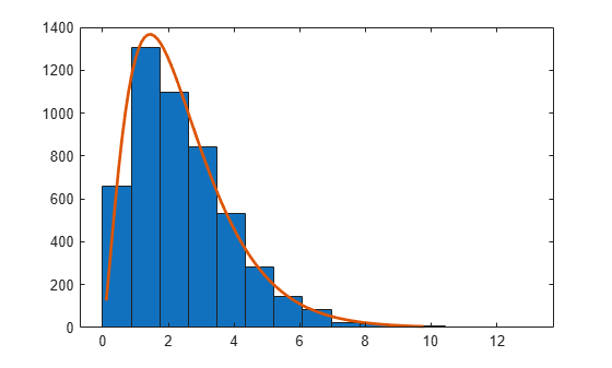

Estimate the second moment of a Gamma distribution by using the sample to perform numerical integration. Compare the result to the theoretical second moment.

x2hat = sum(sample.^2)/numsamples

x2hat = 
8.3104

truex2 = beta^2*gamma(alpha+2)/gamma(alpha)

truex2 = 
8.3349

The estimate is close to the theoretical value.

Explore the convergence rate of the estimate by plotting its evolution.

figure
x2hatchain = cumsum(sample.^2)./(1:numsamples)';
plot(x2hatchain)
hold on
yline(truex2,'--')
title("Second Moment Evolution")

Return Acceptance Rates

Return the acceptance rates for multiple Markov chains.

Create a function that computes the pdf of the Gamma(2.43,1) distribution for an input value.

alpha = 2.43;
beta = 1;
targetPDF = @(x)gampdf(x,alpha,beta);

When you plan to generate multiple chains, ensure that all the custom functions you write and pass to mhsample return a column vector or matrix of values, with each row corresponding to values required by an individual chain. This example uses a univariate, known distribution from which to sample, which simplifies the problem. However, regardless of your functions, you can verify the output by entering test values into each function.

Ensure that the target pdf returns the correct number of pdf evaluations in the correct form.

numchains = 10;
rng(1,"twister")  % For reproducibility
testvalues = gamrnd(alpha,beta,numchains,1);
gold = gampdf(testvalues,alpha,beta);
testtargetpdf = targetPDF(testvalues);
size(testtargetpdf)

ans = 1×2

    10     1

(gold - testtargetpdf)'*(gold - testtargetpdf)

ans = 
0

The true and target pdfs show no difference.

Generate 10 Markov chains of size 5000 samples from the Gamma(2.43,1) distribution using the Random-Walk Metropolis–Hastings sampler with a Gaussian proposal and standard deviation of 10. For each Markov chain, initialize the sampler from a random positive value in (0,1). Return the acceptance rate for each chain.

numsamples = 5000;
start = rand(numchains,1);
[sample,acceptance] = mhsample(start,numsamples,PDF=targetPDF,Proposal="gaussian", ...
    Scale=10,NumChains=numchains);

sample is a 5000-by-10 matrix of samples from the target pdf. Each row is an independent sample. acceptance is a column vector of acceptance rates for each sample.

Create a time series plot of each Markov chain.

figure
h = tiledlayout(4,3);
for j = 1:numchains
    nexttile
    plot(sample(:,:,j))
end
title(h,"Sampled Markov Chains")

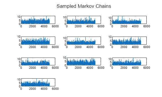
The plots show little transient behavior and almost no serial correlation, indicating that the Markov chains mix well.

Plot the acceptance rates.

figure
plot(acceptance)

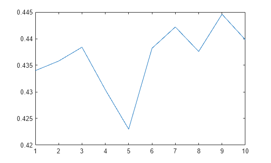
The acceptance rate series is stable, the values are adequate for a Metropolis–Hastings sampler.

Input Arguments

start — Initial values of Markov chain

numeric row vector | numeric matrix

Initial values of the Markov chain, specified as a 1-by-numDims numeric row vector or a numChains-by-numDims numeric matrix.

Column k contains the initial values of random variable k for all generated chains. numDims is the dimension of the random variable to sample.

Row j contains the initial values of all variables for chain j. numChains is the value of the NumChains name-value argument.

Example: Set start to randn(1,5) to specify random standard normal initial values for a distribution with five random variables to sample.

Example: Set start to randn(100,5) and set NumChains=100 to specify random standard normal initial values for a distribution with five random variables to sample, and to generate 100 independent Markov chains.

Data Types: single | double

numsamples — Number of samples to return per Markov chain

positive integer

Number of samples to return per Markov chain, specified as a positive integer.

mhsample generates raw Markov chains of length burnin + thin*numsamples, where burnin and thin are the values of the BurnIn and Thin name-value arguments. Then, mhsample removes the burn-in samples from the raw Markov chain and reduces it by the thinning factor to produce the output chain of length numsamples.

Data Types: single | double

Name-Value Arguments

Specify optional pairs of arguments as Name1=Value1,...,NameN=ValueN, where Name is the argument name and Value is the corresponding value. Name-value arguments must appear after other arguments, but the order of the pairs does not matter.

Example: mhsample(rand(1,5),1000,BurnIn=100,Thin=4) randomly initializes the 5-D random variable by drawing values in [0,1], removes the first 100 draws from the raw generated Markov chain (burn-in period of 100), retains every fourth draw of the remaining chain (thinning factor of 4), and then returns the resulting processed chain of length 1000.

Unlike most MATLAB^® functions, mhsample requires certain name-value arguments.

Target PDF Form (Specify One)

PDF — Target stationary pdf

function handle

Target stationary pdf from which to draw samples, specified as a function handle in the form @fcnName, where fcnName is the function name. You can specify an unnormalized pdf, meaning, the specified pdf can be proportional to the target stationary distribution to sample.

Suppose targetPDF is the name of the MATLAB function defining the target stationary pdf of the numDims-dimensional random variable X. Then, targetPDF must have this form:

function pdf = targetPDF(X)
	...
end

where:

• X is a numChains-by-numDims numeric matrix of the same size and type as start. X contains numChains values of the numDims random variable, from which to evaluate the target stationary pdf.

• pdf is a numChains-by-1 numeric column vector of the target stationary pdf values. pdf(j) is the pdf evaluated at X(j,:).

If you specify PDF, you cannot specify LogPDF.

Example: In mhsample(1,100,PDF=@target,Proposal="gaussian",Scale=100), PDF=@target sets the target pdf to @target, where target is a function for the PDF of the target stationary distribution, from which to generate samples.

Data Types: function_handle

LogPDF — Log density of target stationary probability distribution

function handle

Log density of the target stationary probability distribution from which to draw samples, specified as a function handle in the form @fcnName, where fcnName is the function name. You can specify the log density of an unnormalized pdf, meaning, the associated pdf can be proportional to the target stationary distribution to sample.

Suppose logTargetPDF is the name of the MATLAB function defining the log density of the target stationary probability distribution of the numDims-dimensional random variable X. Then, logTargetPDF must have the form:

function logpdf = logTargetPDF(X)
	...
end

where:

• X is a numChains-by-numDims numeric matrix of the same size and type as start. X contains numChains values of the numDims random variable, from which to evaluate the target stationary pdf.

• logpdf is a numChains-by-1 numeric column vector of the log density values of the target stationary probability distribution. logpdf(j) is the log density evaluated at X(j,:).

If you specify LogPDF, you cannot specify PDF.

Example: In mhsample(rand(1,5),100,LogPDF=@logtarget,Proposal="gaussian",Scale=100), LogPDF=@logtarget sets the log of the target pdf to @logtarget, where logtarget is a function for the log target stationary distribution, from which to generate samples.

Data Types: function_handle

Proposal Random Number Generator (Specify One)

Proposal — Proposal probability distribution name

"gaussian" | "t"

Since R2026a

Proposal probability distribution name, specified as a value in this table.

Value	Description
"gaussian"	Multivariate Gaussian (normal) proposal distribution
"t"	Multivariate Student's t proposal distribution

The center vector of the specified proposal is specified by Center, and the scale matrix is specified by Scale. For Proposal="t", the distribution degrees of freedom is specified by DegreesOfFreedom.

When you specify Proposal:

• You must also specify Scale.

• You cannot specify PropRND, PropPDF, LogPropPDF, or Symmetric.

Tip

The mhsample function shows improved performance when both of the following conditions are true:

• You specify Proposal instead of setting the PropPDF or LogPropPDF name-value argument to a custom function handle to either supported distribution.

• The target distribution evaluation does not dominate overall runtime.

In general, experienced efficiency is problem dependent.

Example: Proposal="gaussian" specifies a Gaussian proposal distribution.

Data Types: char | string

PropRND — Proposal distribution random number generator function

function handle

Proposal distribution random number generator function, specified as a function handle in the form @fcnName, where fcnName is the function name.

Suppose propRND is the name of the MATLAB function defining the proposal random number generator for drawing proposals for the numDims-dimensional random variable X. Then, propRND must have this form.

function nextSample = propRND(X)
	...
end

where:

• X is a numChains-by-numDims numeric matrix of the same size and type as start, representing the current state of all Markov chains.

  When the proposal distribution is independent of the current state of the Markov chain (Independent Metropolis–Hastings), you can specify the placeholder ~ instead of x. For details, see Algorithms.

• nextSample is a numChains-by-numDims numeric matrix of the same size and type as start, containing numChains draws of the numDims random variables from the proposal distribution.

When you specify PropRND:

• You must also specify at least one of the name-value arguments Symmetric, PropPDF, or LogPropPDF.

• You cannot specify Proposal, Center, Scale, or DegreesOfFreedom.

Example: PropRND=@proprnd specifies @proprnd as the function handle to the function that randomly draws from the proposal distribution.

Data Types: function_handle

Proposal Distribution Description (Specify One)

Scale — Scale matrix

positive-definite matrix

Since R2026a

Scale matrix (covariance matrix for a Gaussian proposal) specified as a numDims-by-numDims positive-definite matrix. You must also specify Scale when you specify Proposal. The value of Scale does not apply to custom proposal distributions.

Example: Scale=100 sets the standard deviation of the Gaussian proposal distribution to 100.

Data Types: single | double

Symmetric — Flag indicating whether proposal distribution is symmetric

false (default) | true

Flag indicating whether the custom proposal distribution is symmetric, specified as true or false.

Value	Description	Notes
true	The proposal distribution represented by PropRND is symmetric.	mhsample implements the Random-Walk Metropolis–Hastings algorithm. mhsample ignores the values of PropPDF and LogPropPDF.
false	The proposal distribution represented by PropRND is asymmetric.	If the proposal distribution is independent of the current state of the Markov chain (see Independent Metropolis–Hastings), Symmetric must be false. mhsample requires you to specify either PropPDF or LogPropPDF.

If you specify Symmetric, you cannot specify Proposal, Center, Scale, or DegreesOfFreedom.

Example: mhsample(1,100,PDF=@target,PropRND=@proprnd,Symmetric=true) sets proposalOption to Symmetric=true, indicating that the proposal distribution represented by its random number generating function proprnd is symmetric. Consequently, mhsample implements the Random-Walk Metropolis–Hastings sampler.

Data Types: logical

PropPDF — Proposal pdf

function handle

Proposal pdf, specified as a function handle in the form @fcnName, where fcnName is the function name. You can specify an unnormalized pdf, meaning the specified pdf can be proportional to the proposal.

Suppose propPDF is the name of the MATLAB function defining the proposal pdf of the numDims-dimensional proposal random variable Y. Then, propPDF must have the form:

function pdf = propPDF(Y,X)
	...
end

where:

• Y is a numChains-by-numDims numeric matrix of the same size and type as start. Y contains numChains values of the numDims random variable, from which to evaluate the proposal pdf.

• X represents the current state of the Markov chain, and has the same size and data type as Y.

  When the proposal distribution is independent of the current state of the Markov chain (Independent Metropolis–Hastings), you can specify the placeholder ~ instead of x. For details, see Algorithms.

• pdf is a numChains-by-1 numeric column vector of proposal pdf values. pdf(j) is the pdf evaluated at Y(j).

When you specify PropPDF:

• You cannot specify LogPropPDF, Proposal, Center, Scale, or DegreesOfFreedom.

• The mhsample function ignores PropPDF when Symmetric=true.

Example: mhsample(1,100,PDF=@target,PropRND=@proprnd,PropPDF=@prop) sets the proposal distribution to the custom function prop.

Data Types: function_handle

LogPropPDF — Log density of proposal pdf

function handle

Log density of the proposal pdf, specified as a function handle in the form @fcnName, where fcnName is the function name. You can specify the log density of an unnormalized pdf, meaning the proposal pdf can be proportional to the proposal.

Suppose logPropPDF is the name of the MATLAB function defining the log density of the proposal pdf of the numDims-dimensional proposal random variable Y. Then, logPropPDF must have the form:

function logpdf = logPropPDF(Y,X)
	...
end

where:

• Y is a numChains-by-numDims numeric matrix of the same size and type as start. Y contains numChains values of the numDims random variable, from which to evaluate the log density of the proposal pdf.

• X represents the current state of the Markov chain, and is the same size and data type as Y.

  When the proposal distribution is independent of the current state of the Markov chain (Independent Metropolis–Hastings), you can specify the placeholder ~ instead of x. For details, see Algorithms.

• logpdf is a numChains-by-1 numeric column vector of the log densities. logpdf(j) is the log density evaluated at y(j).

When you specify LogPropPDF:

• You cannot specify PropPDF, Proposal, Center, Scale, or DegreesOfFreedom.

• The mhsample function ignores LogPropPDF when Symmetric=true.

Example: mhsample(1,100,PDF=@target,PropRND=@proprnd,LogPropPDF=@logprop) sets the log of the proposal distribution to the custom function logprop.

Data Types: function_handle

Optional Settings for All Input Argument Combinations

BurnIn — Number of draws to remove from beginning of raw sample

0 (default) | nonnegative scalar

Number of draws to remove from the beginning of the raw sample to reduce transient effects, specified as a nonnegative scalar.

For details on how mhsample reduces the raw sample, see Algorithms.

Example: BurnIn=1000

Data Types: single | double

Thin — Raw sample size multiplier

1 (default) | positive integer

Raw sample size multiplier used to reduce serial correlation in the returned sample, specified as a positive integer.

The raw Monte Carlo sample size is BurnIn + numsamples*Thin. After discarding the burn-in samples, mhsample discards every Thin – 1 draws, and then retains the next draw.

For details on how mhsample reduces the raw sample, see Algorithms.

Example: Thin=4 retains only every fourth draw.

Data Types: single | double

NumChains — Number of independent Markov chains

1 (default) | positive integer

Since R2026a

Number of independent Markov chains to generate, specified as a positive integer.

NumChains must be the same as the number of rows of start.

Example: NumChains=100

Data Types: single | double

Optional Settings Only for Gaussian or Student's t Proposal Distribution

Center — Gaussian or Student's t proposal distribution mean

[] (default) | numeric row vector

Since R2026a

Gaussian or Student's t proposal distribution mean, specified as a 1-by-numDims numeric row vector. To specify Center, you must also specify Proposal.

When you specify Center, mhsample implements the Independent Metropolis–Hastings algorithm, in which successive proposal draws have a distribution with the specified center. Otherwise, mhsample implements the Random-Walk Metropolis–Hastings algorithm, in which successive proposal draws have a distribution centered at the previous accepted draw.

Example: Center=zeros(1,5)

Data Types: single | double

DegreesOfFreedom — Student's t proposal distribution degrees of freedom

5 (default) | positive numeric scalar

Since R2026a

Student's t proposal distribution degrees of freedom, specified as a positive numeric scalar. To specify DegreesOfFreedom, you must also set Proposal to "t".

Example: DegreesOfFreedom=10

Data Types: single | double

Output Arguments

sample — Processed MCMC sample

numeric matrix | numeric array

Processed MCMC samples, returned as a numsamples-by-numDims numeric matrix or a numsamples-by-numDims-NumChains 3-D numeric array. sample(j,k,m) is draw j of variable k in chain m.

mhsample produces the processed MCMC samples by this procedure:

1. Omit the draws in the specified burn-in period BurnIn from the raw sample.

2. Reduce the remaining draws by thinning them using specified thinning factor Thin.

acceptance — Proposal draw acceptance rate

numeric scalar in [0,1] | numeric column vector

Proposal draw acceptance rate for each generated Markov chain, returned as a numeric scalar in the interval [0,1] or a NumChains-by-1 numeric column vector of such values. acceptance(j) is the acceptance rate of Markov chain j.

mhsample computes the acceptance rates from the raw samples (not the samples in sample).

More About

Metropolis–Hastings Sampler

The Metropolis–Hastings sampler is an MCMC method for numerical integration. The goal of the sampler is to draw many random samples from a target probability distribution P(x) (PDF or LogPDF), whose distribution function is known only up to a proportionality constant and, therefore, is difficult to sample. Instead, the sampler draws from a proposal distribution q(x,y) (Proposal or PropRND), a surrogate for the target distribution, whose distribution function is known. The sampler accepts or rejects the draws based on an acceptance probability. After many iterations, a sequence of samples results, forming a Markov chain; asymptotically, the sample is from the stationary distribution of the Markov chain, which is the target distribution.

Statistics and Machine Learning Toolbox™ supports the Random-Walk Metropolis–Hastings and Independent Metropolis–Hastings algorithms. In general, both algorithms follow this procedure, with x₀ = start, the current state of the Markov chain:

1. Draw one observation y from q(y|x_t), the proposal distribution given the current state of the Markov chain x_t.

2. Compute the acceptance probability

   $$r(x_t,y)\text{=}\text{}\min \left(\frac{f(y)}{f(x_t)}\frac{q(x_t|y)}{q(y|x_t)},\text{}1\right).$$

3. Draw u ~ Uniform(0,1).

4. If r(x_t,y) ≥ u, accept the proposal and set the next state of the Markov chain to x_{t + 1} = y. Otherwise, reject the proposal and keep the current state by setting x_{t + 1} = x_t.

5. Iterate steps 1 through 4 BurnIn + numsamples*Thin times.

The quality of the sample and the efficiency of the algorithm depend on how well the proposal distribution approximates the target.

Random-Walk Metropolis–Hastings Sampler

The proposal distribution q of the Random-Walk Metropolis–Hastings sampler is dependent on the current state of the Markov chain x_t.

Usually, the conditional proposal distribution has the general form q(y|x_t) = x_t + ε_t, where ε_t is random symmetric error. This form shows the association with past draws, a feature of a random walk. Consequently, the resulting sample (Markov chain) can have significant serial correlation.

Independent Metropolis–Hastings Sampler

The proposal distribution q of the Independent Metropolis–Hastings sampler is independent of the current state of the Markov chain x_t. Symbolically, q(y|x_t) = q(y).

Tips

• When you plan to return multiple independent samples by using the NumChains name-value argument, ensure that all custom functions you pass to mhsample return a numeric column vector or matrix of values, with each row corresponding to the values required by the corresponding Markov chain. The noncustom proposal distributions, available with the Proposal name-value argument, enable you to avoid writing custom functions which might not return values in the correct form for multiple Markov chains. The noncustom proposal distributions are easy to use, provide increased sampling speed compared to custom proposals, can be tuned easily, and work well for a variety of applications. Therefore, a good practice is to try setting Proposal before writing and setting custom proposal distributions.

• An acceptance rate close to 0 indicates that most proposal draws likely correspond to regions of low probability in the target distribution. An acceptance rate close to 1 can indicate that the proposal draws do not sufficiently explore the target distribution. However, an ideal acceptance rate depends on the target distribution. In general, Gelman, et al, suggest tuning the sampler until the acceptance rate is close to 0.25[1].

Algorithms

mhsample implements the Random-Walk or Independent Metropolis–Hastings sampler algorithm depending on your specifications.

Algorithm	Specifications
Random-Walk Metropolis–Hastings	mhsample implements this algorithm when you specify any one of these name-value argument combinations: Proposal=proposal,Scale=scale,...otherOptions..., where otherOptions excludes Center PropRND=propRND,Symmetric=true,...otherOptions... PropRND=propRND,PropPDF=propPDF,...otherOptions..., where propPDF depends on the current state of the Markov chain PropRND=propRND,LogPropPDF=logPropPDF,...otherOptions..., where logPropPDF depends on the current state of the Markov chain
Independent Metropolis–Hastings	mhsample implements this algorithm when you specify any one of these name-value argument combinations: Proposal=proposal,Scale=scale,Center=center...otherOptions... PropRND=propRND,PropPDF=propPDF,...otherOptions..., where propPDF is independent of the current state of the Markov chain, and Symmetric is false (the default) PropRND=propRND,LogPropPDF=logPropPDF,...otherOptions..., where logPropPDF is independent of the current state of the Markov chain and Symmetric is false When using the custom proposal functions propRND, propPDF, and logPropPDF, you can use the placeholder ~ for input that corresponds to the current state of the Markov chain. The placeholder reserves the input position but takes no effect in the function.

For each of NumChains generated Markov chains, mhsample draws BurnIn + Thin*numsamples samples, and then processes each sample by removing the burn-in draws specified by BurnIn, and then reducing the remaining draws as specified by the thinning factor Thin.

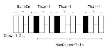
This figure illustrates how mhsample reduces the raw MCMC sample. Rectangles represent successive draws from the distribution. mhsample removes the white rectangles from the Monte Carlo sample. The remaining numsamples black rectangles compose sample.

References

[1] Gelman, Andrew, Walter R. Gilks, and Gareth O. Roberts. "Weak Convergence and Optimal Scaling of Random Walk Metropolis Algorithms." The Annals of Applied Probability. 7 (February 1997): 110–120. https://doi.org/10.1214/aoap/1034625254.

Version History

Introduced in R2006a

R2026a: For improved performance, explicitly specify a Gaussian or Student's t proposal distribution

The Proposal name-value argument enables you to explicitly specify a Gaussian or Student's t proposal distribution. You can tune the sampler by adjusting corresponding distribution parameters using name-value argument syntax.

Name	Proposal Distribution	Parameters
"gaussian"	Multivariate Gaussian distribution	Center — Optional mean vector Scale — Required covariance matrix
"t"	Multivariate Student's t distribution	Center — Optional center vector Scale — Required scale matrix DegreesOfFreedom — Optional degrees of freedom

The mhsample function shows improved performance when both of the following are true:

• You specify a Gaussian or Student's t proposal distribution by using Proposal instead of setting the PropPDF or LogPropPDF name-value argument to a custom function handle to either distribution.

• The target distribution evaluation does not dominate overall run time.

In general, experienced efficiency is problem dependent.

The code below compares the run-time performance of mhsample when you implicitly specify a scale 1 Gaussian proposal distribution by using a custom function to the performance when you explicitly specify a scale 1 Gaussian proposal by using the Proposal and Scale name-value arguments.

F  = @(x) -x.^2 + log(2 + sin(5*x) + sin(2*x)); % Target stationary distribution log PDF
numSamples = 500000;                            % Length of the MCMC chain
propPDF = @(x,y)mvnpdf(x,y,1);                  % Proposal probability density function
propRNG = @(x)mvnrnd(x,1);                      % Proposal random number generator

% Implicitly specify a Gaussian proposal by specifying a function handle 
% to a Gaussian random number generator.
rng(1,"twister")
timeitimplicit = @()mhsample(0,numSamples,LogPDF=F,PropPDF=propPDF, ...
    PropRND=propRNG,Symmetric=true);
timecgp = timeit(timeitimplicit);

% Explicitly specify a Gaussian proposal, under the same conditions, by naming 
% the proposal distribution using Proposal.
rng(1,"twister")
timeitexplicit = @()mhsample(0,numSamples,LogPDF=F,Proposal="Gaussian", ...
    Scale=1);
timegp = timeit(timeitexplicit);

R2026a, implicit Gaussian proposal specification using function handle: 0.45 sec

R2026a, explicit Gaussian proposal specification using Proposal argument: 8.83 sec

The mhsample function is 20x faster when a Gaussian proposal is explicitly specified. The code was timed on a Windows 11 Enterprise, Intel(R) Xeon(R) W-2133 CPU @ 3.60GHz 3.60 GHz system.

R2026a: NumChains name-value argument replaces nchains

To specify the number of Markov chains to generate from the Metropolis–Hasting algorithm, use the NumChains name-value argument instead of nchains. Although you should update your code to use NumChains instead of nchains, there are no plans to remove nchains.