Custom Inductor (B-H Curve)
This example shows a comparison in behavior of a linear and nonlinear inductor. Starting with fundamental parameter values, the parameters for linear and nonlinear representations are derived. These parameters are then used in a Simscape™ model and the simulation outputs compared.
Open Model

Specification of Parameters
Fundamental parameter values used as the basis for subsequent calculations:
Permeability of free space,

Relative permeability of core,

Number of winding turns,

Effective magnetic core length,

Effective magnetic core cross-sectional area,

Core saturation begins,

Core fully saturated,

Calculate Magnetic Flux Density and Magnetic Field Strength Data
Where:
Magnetic flux density,

Magnetic field strength,

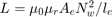
Linear representation:

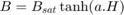
Nonlinear representation (including coefficient, a):
Display Magnetic Flux Density Versus Magnetic Field Strength
The linear and nonlinear representations can be overlaid.

Calculate Magnetic Flux and Current Data
Where:
Magnetic flux,

Current,

Linear representation:

Nonlinear representation:


Display Magnetic Flux Versus Current
The linear and nonlinear representations can be overlaid.

Use Parameters in Simscape Model
The parameters calculated can now be used in a Simscape model. Once simulated, the model is set to create a Simscape logging variable, simlog_CustomInductorBHCurve.
Conclusion
The state variable for both representations is magnetic flux,  . Current, I, and magnetic flux, , can be obtained from the Simscape logging variable, simlog_CustomInductorBHCurve, for each representation. Overlaying the simulation results from the representations permits direct comparison.

Results from Real-Time Simulation
This example has been tested on these platforms:
Speedgoat™ Performance real-time target machine with an Intel® 3.5 GHz i7 multi-core CPU and 4 GB RAM.
dSPACE® SCALEXIO LabBox with Intel® Core XEON E3-1275v3 at 3.5GHz and 4 GB RAM.
You can run this model in real time with a step size of 10 microseconds by using the Simscape local solver. For small sample rates, a task overrun might occur during the initial task execution due to a cold cache. To avoid this overrun, if the selected platform supports these options, relax the start-up behavior by specifying a limited number of task overruns or increasing the sample time of periodic tasks during the start-up phase of the real-time application.