Constrain a Point to a Curve
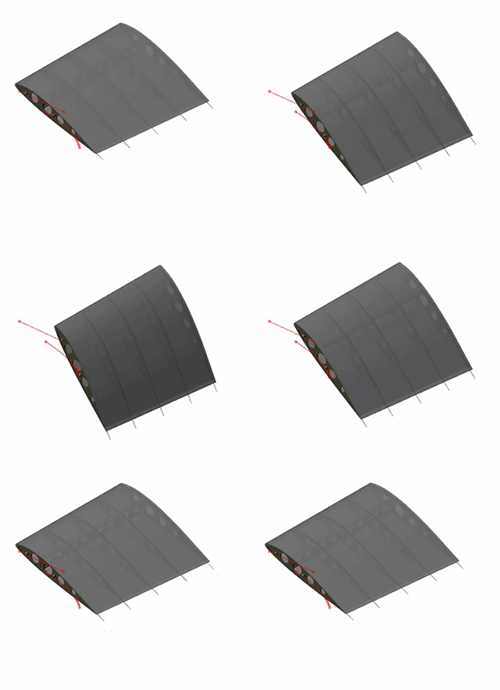
This example shows how to apply multiple point-on-curve constraints to a single body. The example is based on a partial model of an aircraft flap that extends and retracts by riding on curved tracks. You complete the multibody dynamics model by adding point-on-curve constraints between two points on the flap and the flap track curves. The figure shows the visualization results of the flap model, once it is complete.
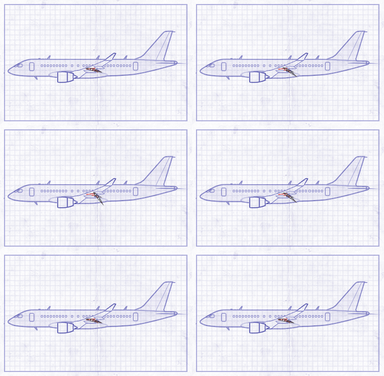
Open the Flap Assembly Model
To open the flap assembly model, at the MATLAB® command prompt, enter:
open_system("DocPocFlapStart")
Save the model with a different name in a convenient folder so that you do not inadvertently overwrite the model.
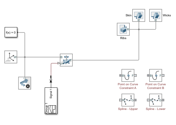
The model is missing key connection lines and block parameters and does yet not simulate. Three rigidly connected blocks, named Ribs, Skin, and Wicks, represent the flap body. A Planar Joint block connects this body to the world frame with three degrees of freedom—one rotational and two translational.
Effect of Constraints on the Model
The flap is at this point unconstrained. In this state, the degrees of freedom of the flap are those provided by the Planar Joint block. The flap is free to rotate about the z-axis, translate along the x-axis, and translate along the y-axis. The animated figure shows these motions. The frame axes are color-coded, with red denoting x, green y, and blue z. The z-axis points out of the screen is not visible in the figure.
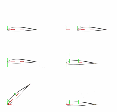
The point-on-curve constraints couple the initially independent motions of the flap so that any one of these motions suffices to completely determine the flap trajectory. For example, in the fully constrained flap, a translation along the x-axis determines also the translation along the y-axis and the rotation about the z-axis. The animated figure shows the constrained motion that you obtain at the end of this example.

Create the Connection Frames
In the Ribs File Solid block dialog box, expand the Frames node and click the
 button. The frame creation interface opens. You use this interface to create a new frame and set its position and orientation with respect to the solid geometry.
In the visualization pane, zoom in on the top portion of the flap and select the top surface of the rightmost cylindrical protrusion, as shown in the figure. The visualization pane highlights the selected surface and reveals its normal vector.
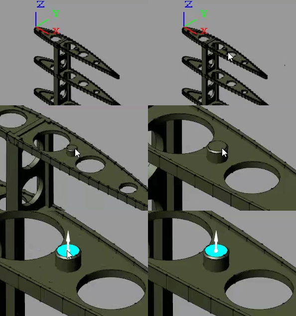
In the Frame Origin area of the frame creation interface, click the Based on Geometric Feature radio button and then the Use Selected Feature button. The frame moves to the center of the selected surface.
Click the Save button to add the new frame to the solid. The block exposes a new port, F1, corresponding to the new frame. You can rename the frame anything you want but, in this example, the default name suffices.
Repeat above steps to create a second frame with origin at the top surface of the leftmost cylindrical protrusion, as shown in the figure. The block exposes a new port, F2, corresponding to the new frame.

Connect the Constraint Blocks
Connect the frame port of each Spline block to the World Frame block. This connection ensures that the constraint curves specified in the Spline blocks are resolved in the World frame. The curve definitions are currently the block defaults. You later change these defaults to obtain a reasonable flap trajectory.
Connect the frame ports of the Point on Curve Constraint blocks to the frame ports that you added to the Ribs File Solid block (F1 and F2). The origins of these frames are the points that you constrain in this example.
Connect the geometry ports of the Spline blocks to the geometry ports of the Point on Curve Constraint blocks as shown in the figure. The geometry connection lines identify the spline curve definitions as the curves to constrain.

Specify the Flap Constraint Curves
Open Model Explorer and, in the Model Hierarchy pane, expand the DocPocFlapStart > Model Workspace node. Model Explorer enables you to define workspace variables so that you can reference them in block dialog box parameters.
In the Model Workspace pane of Model Explorer, set the Data source parameter to
MATLAB Code. An editable field appears with the still-incomplete variable definitions:
theta = linspace(4*pi/12,pi/8,4)';
lowerTrack = [];
upperTrack = [];
The variables
lowerTrackandupperTrackare the constraint curves of the lower and upper flap tracks. The variablethetais an angle range used in the definition of the lower track curve.Complete the
lowerTrackandupperTrackdefinitions by specifying a few points on the curves as shown in the following code snippet. You must click the Reinitialize from Source button to apply the changes to the model. The new code portions are shown in blue.
theta = linspace(4*pi/12,pi/8,4)';
lowerTrack = [350 0; (640+100*cos(theta)) (130*sin(theta)-210)];
upperTrack = [50 50; 550 100];
In the dialog box of each Spline block, specify the parameters listed in the table. The Interpolation Points parameter is defined in terms of the MATLAB variables from the model workspace. Ensure that this parameter is in units of
mm. The Color parameter is defined as a normalized RGB vector corresponding to a light shade of red.

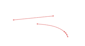
Update the block diagram. In the Modeling tab, click Update Model. Multibody Explorer opens with a static visualization of the model in its initial configuration. The figure shows the spline curves as they appear in Multibody Explorer with the bodies hidden. You can hide a body by selecting its node in the Model Tree pane and selecting Hide This.
Simulate the Model
Simulate the model. Multibody Explorer shows a dynamic visualization of the flap assembly. The motion of the flap is now constrained so that the origins of the frames you created always lie on the curves you defined. Switch between the standard views of Multibody Explorer or rotate, pan, and zoom to better explore the flap and its motion.
To open a complete version of the flap assembly model, at the MATLAB command prompt, enter:
open_system("DocPocFlap")