Using Modal Reduction in Flexible Bodies to Improve Simulation Performance

This example shows how you can use modal reduction for performance acceleration in models with flexible bodies. The model in this example uses a rectangular beam for simplicity, but you can apply modal reduction to all flexible body blocks. By only retaining the lowest-frequency modes of vibration of flexible bodies in your multibody system, you can speed up simulation while maintaining sufficient fidelity.

To have the best reading experience of this example, you can hide the code. To hide the code, you can go to the View tab, and in the View section, click Hide Code . If plots and tables do not display, you can go to the Live Editor tab and click Run .

Modal Reduction Study of Cantilever Beam

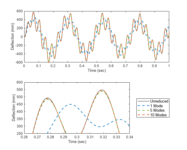
This example investigates the response of a cantilever beam when a sinusoidal force is applied to its free end. You can perform a comparative study of the results obtained when the model is unreduced, and when the model retains the first 1, 5 and 10 modes. For more information on the model, check the file ModalReductionForFlexibleBodies.slx in the Current Folder browser.

numModes = [1 5 10];
 
[simTimeUnred,simTimesRed] = simulateAndPlot(numModes);

The figure shows the transverse deflection of the free end of the beam. The upper subplot shows the simulation output, while the lower subplot zooms in on a short time interval for clarity. The plots show that only a few of the lowest-frequency modes are needed to capture the bulk of the flexible body's behavior in this scenario.

The table shows the simulation times for the different cases as well as the improvement in performance compared to the unreduced simulation:

[numModes,sortIndices] = sort(numModes,"descend");
simTimesRed = simTimesRed(sortIndices);
disp(table( ...
    ["Unreduced";numModes(:)], ...
    [string(num2str([simTimeUnred;simTimesRed(:)],"%6.3f"))], ...
    [" - ";string(num2str(simTimeUnred./simTimesRed(:),"%4.1fx"))], ...
    'VariableNames',["Number of Modes", ...
                     "Simulation Time (sec)", ...
                     "Performance Improvement"]));

    Number of Modes    Simulation Time (sec)    Performance Improvement
    _______________    _____________________    _______________________

      "Unreduced"             "3.116"                   " - "          
      "10"                    "0.756"                   " 4.1x"        
      "5"                     "0.400"                   " 7.8x"        
      "1"                     "0.250"                   "12.5x"        

Specify Number of Modes

Enter the number of modes you want to retain, then run the analysis to perform a comparison against the unreduced case.

maxNumModes = getMaxNumModes();
numModes = 5;  
[simTimeUnred,simTimesRed] = simulateAndPlot(numModes);

fprintf("It took %.3f sec to simulate the unreduced model, and\n" + ...
        "%.3f sec for the reduced model, which is %.1fx faster.", ...
        simTimeUnred,simTimesRed,round(simTimeUnred./simTimesRed,1));

It took 3.565 sec to simulate the unreduced model, and
0.395 sec for the reduced model, which is 9.0x faster.

function maxNumModes = getMaxNumModes()
% Helper function to determine the maximum possible number of modes that can be
% requested based on the number of beam finite elements in the cantilever beam
% model.

    % Setup
    model = "ModalReductionForFlexibleBodies";
    load_system(model);
    beamPath = model + "/Beam";

    % Infer the maximum number of modes from the number of beam elements
    numElements = str2double(get_param(beamPath,"NumElements"));
    maxNumModes = 6*numElements;

    % Teardown
    close_system(model,0);

end


function [simTimeUnred,simTimesRed] = simulateAndPlot(numModesVec)
% Helper function to simulate the cantilever beam model and plot its tip
% deflection, without modal reduction as well as with modal reduction, using the
% given values for the number of retained modes.

    % Setup
    model = "ModalReductionForFlexibleBodies";
    load_system(model);
    set_param(model,"SimMechanicsOpenEditorOnUpdate","off");
    beamPath = model + "/Beam";

    % Simulate the model without modal reduction
    set_param(beamPath,"ReductionType","None");
    simOut = sim(model,"ReturnWorkspaceOutputs","on");
    simTimeUnred = simOut.SimulationMetadata.TimingInfo.ExecutionElapsedWallTime;

    % Create a new window figure
    figure("Units","normalized","Position",[0 0 0.5 0.5]);
    colororder(["#7E2F8E","#0072BD","#77AC30","#D95319","#4DBEEE","#EDB120","#A2142F"]);

    % Plot the beam's tip deflection response
    subplot(2,1,1);
    plot(simOut.tout,simOut.z,"k-","DisplayName","Unreduced");
    xlim([0 1]);
    xlabel("Time (sec)","FontSize",10);
    ylim([-600 600]);
    ylabel("Deflection (mm)","FontSize",10);
    hold on 

    % Plot the same response, but zoomed in
    subplot(2,1,2);
    plot(simOut.tout,simOut.z,"k-","DisplayName","Unreduced");
    xlim([0.26 0.34]);
    xlabel("Time (sec)","FontSize",10);
    ylim([250 600]);
    ylabel("Deflection (mm)","FontSize",10);
    legend("Location","eastoutside","FontSize",10);
    hold on

    % Update the figure window
    drawnow

    % Simulate and plot the results with modal reduction
    set_param(beamPath,"ReductionType","ModallyReduced");
    set_param(beamPath,"NumRetainedModes",num2str(1));
    sim(model); % May help improve timing results
    N = numel(numModesVec);
    simTimesRed = zeros(1,N);
    for i = 1:N
        % Simulate the model with modal reduction
        numModes = numModesVec(i);
        set_param(beamPath,"NumRetainedModes",num2str(numModes));
        simOut = sim(model,"ReturnWorkspaceOutputs","on");
        simTimesRed(i) = simOut.SimulationMetadata.TimingInfo.ExecutionElapsedWallTime;

        % Plot the beam's tip deflection response
        numModesStr = numModes + " Mode";
        if numModes > 1
            numModesStr = numModesStr + "s";
        end
        subplot(2,1,1);
        plot(simOut.tout,simOut.z,"--","LineWidth",1.5,"DisplayName",numModesStr);
        subplot(2,1,2);
        plot(simOut.tout,simOut.z,"--","LineWidth",1.5,"DisplayName",numModesStr);

        % Update the figure window
        drawnow
    end

    % Teardown
    close_system(model,0);

end