Engine Speed Model Parameter Estimation

This example shows how to estimate the coefficients of a nonlinear (quadratic) function to approximate the dynamic behavior of a system component.

Description of the Engine Speed Model

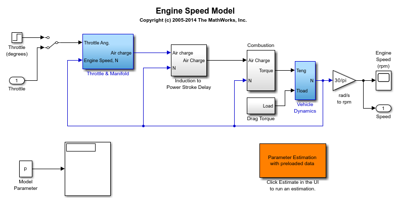
The Simulink® model for the engine system, spe_speed, is shown below.

The throttle angle from the block labeled "Throttle" on the left side of the diagram drives the simulation. The output of interest in the model is the engine speed, which can be monitored by opening the Scope block labeled "Engine Speed (rpm)".

Open the engine speed model.

open_system('spe_speed')

Modeling Air Charge Using a Nonlinear Function

Among other dynamic components in the model, the "Intake Manifold" subsystem is used to model the dynamics of the air intake manifold in the engine.

Open the Intake Manifold subsystem.

open_system('spe_speed/Throttle & Manifold/Intake Manifold')

In particular, the "Convert to mass charge" block above defines a quadratic multi-variable polynomial to approximate the relationship between the Air Charge, the Manifold Pressure, and the Engine Speed. This approximation has the following form:

The Parameter Estimation Problem

When measured data for various signals in your model are available, you can use Simulink® Design Optimization™ to compute the unknown parameters.

The parameter estimation problem in our case is to compute the coefficients

using measured data.

You can launch a pre-configured parameter estimation task in the Parameter Estimator by first opening the model and by double-clicking on the orange block in the lower corner of the model.