Tuning Multiloop Control Systems
This example shows how to jointly tune the inner and outer loops of a cascade simulink architecture with the systune command.
Cascaded PID Loops
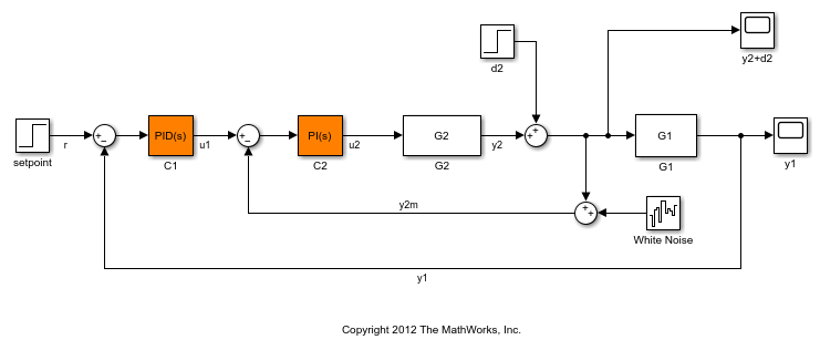
Cascade control is often used to achieve smooth tracking with fast disturbance rejection. The simplest cascade architecture involves two control loops (inner and outer) as shown in the block diagram below. The inner loop is typically faster than the outer loop to reject disturbances before they propagate to the outer loop.
open_system('rct_cascade')
Plant Models and Bandwidth Requirements
In this example, the inner loop plant G2 is

and the outer loop plant G1 is
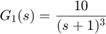
G2 = zpk([],-2,3);
G1 = zpk([],[-1 -1 -1],10);
We use a PI controller in the inner loop and a PID controller in the outer loop. The outer loop must have a bandwidth of at least 0.2 rad/s and the inner loop bandwidth should be ten times larger for adequate disturbance rejection.
Tuning the PID Controllers with SYSTUNE
When the control system is modeled in Simulink, use the slTuner interface in Simulink Control Design™ to set up the tuning task. List the tunable blocks, mark the signals r and d2 as inputs of interest, and mark the signals y1 and y2 as locations where to measure open-loop transfers and specify loop shapes.
ST0 = slTuner('rct_cascade',{'C1','C2'});
addPoint(ST0,{'r','d2','y1','y2'})
You can query the current values of C1 and C2 in the Simulink model using showTunable. The control system is unstable for these initial values as confirmed by simulating the Simulink model.
showTunable(ST0)
Block 1: rct_cascade/C1 =

             1
  Kp + Ki * ---
             s

  with Kp = 0.1, Ki = 0.1

Name: C1
Continuous-time PI controller in parallel form.

-----------------------------------

Block 2: rct_cascade/C2 =

             1
  Kp + Ki * ---
             s

  with Kp = 0.1, Ki = 0.1

Name: C2
Continuous-time PI controller in parallel form.
Next use "LoopShape" requirements to specify the desired bandwidths for the inner and outer loops. Use  as the target loop shape for the outer loop to enforce integral action with a gain crossover frequency at 0.2 rad/s:
% Outer loop bandwidth = 0.2
s = tf('s');
Req1 = TuningGoal.LoopShape('y1',0.2/s); % loop transfer measured at y1
Req1.Name = 'Outer Loop';
Use  for the inner loop to make it ten times faster (higher bandwidth) than the outer loop. To constrain the inner loop transfer, make sure to open the outer loop by specifying
 y1 as a loop opening:
% Inner loop bandwidth = 2
Req2 = TuningGoal.LoopShape('y2',2/s); % loop transfer measured at y2
Req2.Openings = 'y1';                  % with outer loop opened at y1
Req2.Name = 'Inner Loop';
You can now tune the PID gains in C1 and C2 with systune:
ST = systune(ST0,[Req1,Req2]);
Final: Soft = 0.859, Hard = -Inf, Iterations = 69
Use showTunable to see the tuned PID gains.
showTunable(ST)
Block 1: rct_cascade/C1 =

             1            s
  Kp + Ki * --- + Kd * --------
             s          Tf*s+1

  with Kp = 0.0521, Ki = 0.0187, Kd = 0.0477, Tf = 0.00594

Name: C1
Continuous-time PIDF controller in parallel form.

-----------------------------------

Block 2: rct_cascade/C2 =

             1
  Kp + Ki * ---
             s

  with Kp = 0.719, Ki = 1.23

Name: C2
Continuous-time PI controller in parallel form.
Validating the Design
The final value is less than 1 which means that systune successfully met both loop shape requirements. Confirm this by inspecting the tuned control system ST with viewGoal.
viewGoal([Req1,Req2],ST)
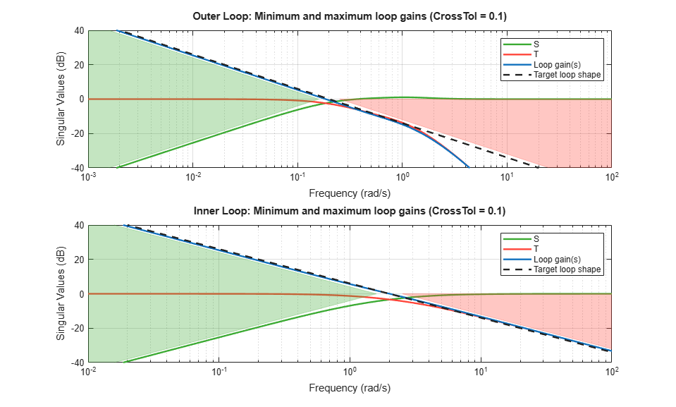
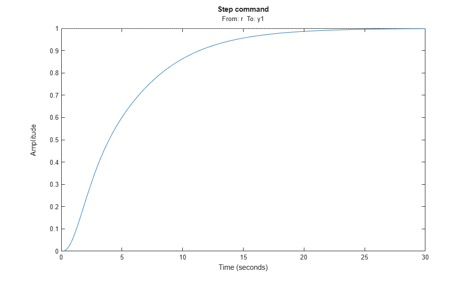
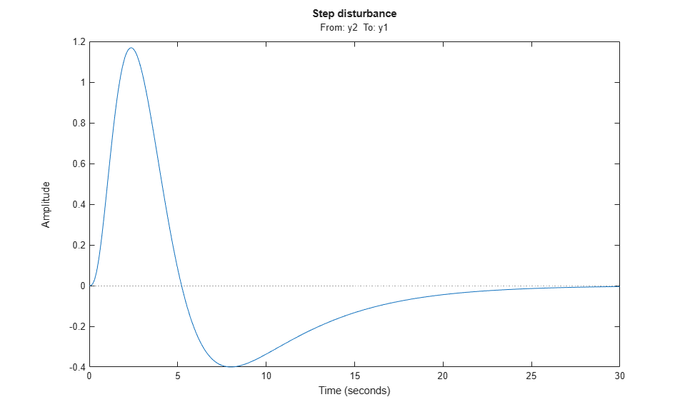
Note that the inner and outer loops have the desired gain crossover frequencies. To further validate the design, plot the tuned responses to a step command r and step disturbance d2:
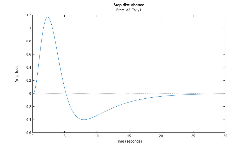
% Response to a step command
H = getIOTransfer(ST,'r','y1');
clf, step(H,30), title('Step command')
% Response to a step disturbance
H = getIOTransfer(ST,'d2','y1');
step(H,30), title('Step disturbance')
Once you are satisfied with the linear analysis results, use writeBlockValue to write the tuned PID gains back to the Simulink blocks. You can then conduct a more thorough validation in Simulink.
writeBlockValue(ST)
Equivalent Workflow in MATLAB
If you do not have a Simulink model of the control system, you can perform the same steps using LTI models of the plant and Control Design blocks to model the tunable elements.
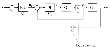
Figure 1: Cascade Architecture
First create parametric models of the tunable PI and PID controllers.
C1 = tunablePID('C1','pid');
C2 = tunablePID('C2','pi');
Then use "analysis point" blocks to mark the loop opening locations y1 and y2.
LS1 = AnalysisPoint('y1');
LS2 = AnalysisPoint('y2');
Finally, create a closed-loop model T0 of the overall control system by closing each feedback loop. The result is a generalized state-space model depending on the tunable elements C1 and C2.
InnerCL = feedback(LS2*G2*C2,1);
T0 = feedback(G1*InnerCL*C1,LS1);
T0.InputName = 'r';
T0.OutputName = 'y1';
You can now tune the PID gains in C1 and C2 with systune.
T = systune(T0,[Req1,Req2]);
Final: Soft = 0.86, Hard = -Inf, Iterations = 116
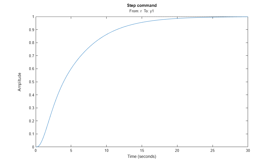
As before, use getIOTransfer to compute and plot the tuned responses to a step command r and step disturbance entering at the location y2:
% Response to a step command
H = getIOTransfer(T,'r','y1');
clf, step(H,30), title('Step command')
% Response to a step disturbance
H = getIOTransfer(T,'y2','y1');
step(H,30), title('Step disturbance')
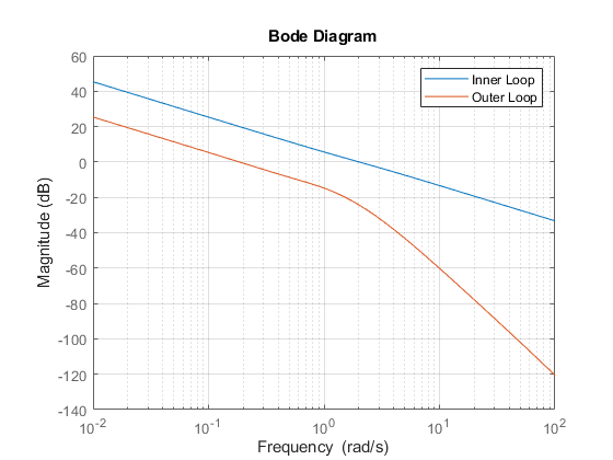
You can also plot the open-loop gains for the inner and outer loops to validate the bandwidth requirements. Note the -1 sign to compute the negative-feedback open-loop transfer:
L1 = getLoopTransfer(T,'y1',-1);       % crossover should be at .2
L2 = getLoopTransfer(T,'y2',-1,'y1');  % crossover should be at 2
bodemag(L2,L1,{1e-2,1e2}), grid
legend('Inner Loop','Outer Loop')