Tune Control Systems in Simulink
This example shows how to use systune or looptune to automatically tune control systems modeled in Simulink®.
Engine Speed Control
For this example we use the following model of an engine speed control system:
open_system('rct_engine_speed')
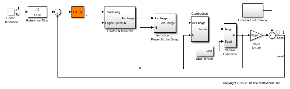
The control system consists of a single PID loop and the PID controller gains must be tuned to adequately respond to step changes in the desired speed. Specifically, we want the response to settle in less than 5 seconds with little or no overshoot. While pidtune is a faster alternative for tuning a single PID controller, this simple example is well suited for an introduction to the systune and looptune workflows in Simulink.
Controller Tuning with SYSTUNE
The slTuner interface provides a convenient gateway to systune for control systems modeled in Simulink. This interface lets you specify which blocks in the Simulink model are tunable and what signals are of interest for open- or closed-loop validation. Create an slTuner instance for the rct_engine_speed model and list the "PID Controller" block (highlighted in orange) as tunable. Note that all Linear Analysis points in the model (signals "Ref" and "Speed" here) are automatically available as points of interest for tuning.
ST0 = slTuner('rct_engine_speed','PID Controller');
The PID block is initialized with its value in the Simulink model, which you can access using getBlockValue. Note that the proportional and derivative gains are initialized to zero.
getBlockValue(ST0,'PID Controller')
ans =

        1
  Ki * ---
        s

  with Ki = 0.01

Name: PID_Controller
Continuous-time I-only controller.
Next create a step tracking requirement to capture the target settling time of 5 seconds. Use the signal names in the Simulink model to refer to the reference and output signals, and specify the target response as a first-order response with time constant of 1 second.
TrackReq = TuningGoal.StepTracking('Ref','Speed',1);
You can now tune the control system ST0 subject to the requirement TrackReq.
ST1 = systune(ST0,TrackReq);
Final: Soft = 0.282, Hard = -Inf, Iterations = 65
The final value is close to 1 indicating that the tracking requirement is met. systune returns a "tuned" version ST1 of the control system described by ST0. Again use getBlockValue to access the tuned values of the PID gains:
getBlockValue(ST1,'PID Controller')
ans =

             1            s
  Kp + Ki * --- + Kd * --------
             s          Tf*s+1

  with Kp = 0.00217, Ki = 0.00341, Kd = 0.000513, Tf = 1.56e-06

Name: PID_Controller
Continuous-time PIDF controller in parallel form.
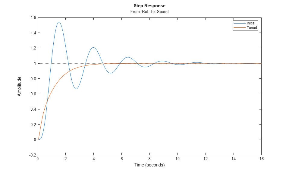
To simulate the closed-loop response to a step command in speed, get the initial and tuned transfer functions from speed command "Ref" to "Speed" output and plot their step responses:
T0 = getIOTransfer(ST0,'Ref','Speed');
T1 = getIOTransfer(ST1,'Ref','Speed');
step(T0,T1)
legend('Initial','Tuned')
Controller Tuning with LOOPTUNE
You can also use looptune to tune control systems modeled in Simulink. The looptune workflow is very similar to the systune workflow. One difference is that looptune needs to know the boundary between the plant and controller, which is specified in terms of controls and measurements signals. For a single loop the performance is essentially captured by the response time, or equivalently by the open-loop crossover frequency. Based on first-order characteristics the crossover frequency should exceed 1 rad/s for the closed-loop response to settle in less than 5 seconds. You can therefore tune the PID loop using 1 rad/s as target 0-dB crossover frequency.
% Mark the signal "u" as a point of interest
addPoint(ST0,'u')

% Tune the controller parameters
Control = 'u';
Measurement = 'Speed';
wc = 1;
ST1 = looptune(ST0,Control,Measurement,wc);
Final: Peak gain = 0.93, Iterations = 5
Achieved target gain value TargetGain=1.
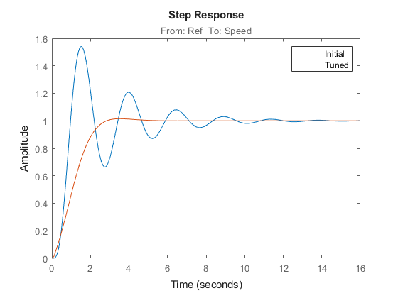
Again the final value is close to 1, indicating that the target control bandwidth was achieved. As with systune, use getIOTransfer to compute and plot the closed-loop response from speed command to actual speed. The result is very similar to that obtained with systune.
T0 = getIOTransfer(ST0,'Ref','Speed');
T1 = getIOTransfer(ST1,'Ref','Speed');
step(T0,T1)
legend('Initial','Tuned')
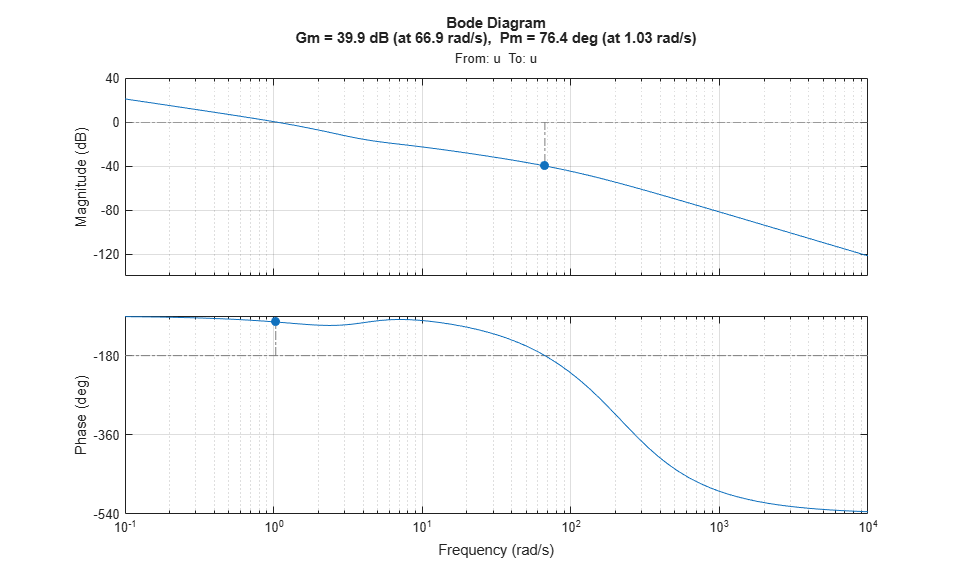
You can also perform open-loop analysis, for example, compute the gain and phase margins at the plant input u.
% Note: -1 because |margin| expects the negative-feedback loop transfer
L = getLoopTransfer(ST1,'u',-1);

margin(L), grid
Validation in Simulink
Once you are satisfied with the systune or looptune results, you can upload the tuned controller parameters to Simulink for further validation with the nonlinear model.
writeBlockValue(ST1)
You can now simulate the engine response with the tuned PID controller.
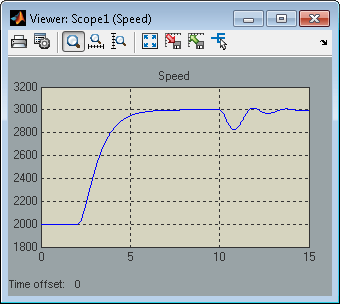
The nonlinear simulation results closely match the linear responses obtained in MATLAB®.
Constraints on PID Gains
It is often useful to constrain the range of tuned parameters to weed out undesirable solutions. For example, you may require that the proportional and derivative gains of the PID controller be nonnegative. To do this, access the tuned block parameterization.
C = getBlockParam(ST0,'PID Controller')
Tunable continuous-time PID controller "PID_Controller" with formula:

             1            s
  Kp + Ki * --- + Kd * --------
             s          Tf*s+1

and tunable parameters Kp, Ki, Kd, Tf.

Type "pid(C)" to see the current value.
Set the "Minimum" value of the tunable parameters Kp and Kd to 0.
C.Kp.Minimum = 0;
C.Kd.Minimum = 0;
Finally, associate the modified parameterization with the tuned block.
setBlockParam(ST0,'PID Controller',C)
Retune the PID gains and verify that the proportional and derivative gains are indeed nonnegative.
ST1 = looptune(ST0,Control,Measurement,wc);

showTunable(ST1)
Final: Peak gain = 0.949, Iterations = 4
Achieved target gain value TargetGain=1.

Block 1: rct_engine_speed/PID Controller =

             1            s
  Kp + Ki * --- + Kd * --------
             s          Tf*s+1

  with Kp = 0.000884, Ki = 0.00332, Kd = 0.000218, Tf = 0.01

Name: PID_Controller
Continuous-time PIDF controller in parallel form.
Comparison of PI and PID Controllers
Closer inspection of the tuned PID gains suggests that the contribution of the derivative term is minor. This suggests using a simpler PI controller instead. To do this, override the default parameterization for the "PID Controller" block:
setBlockParam(ST0,'PID Controller',tunablePID('C','pi'))
This specifies that the "PID Controller" block should now be parameterized as a mere PI controller. Next re-tune the control system for this simpler controller:
ST2 = looptune(ST0,Control,Measurement,wc);
Final: Peak gain = 0.95, Iterations = 4
Achieved target gain value TargetGain=1.
Again the final value is less than one indicating success. Compare the closed-loop response with the previous ones:
T2 = getIOTransfer(ST2,'Ref','Speed');
step(T0,T1,T2,'r--')
legend('Initial','PID','PI')
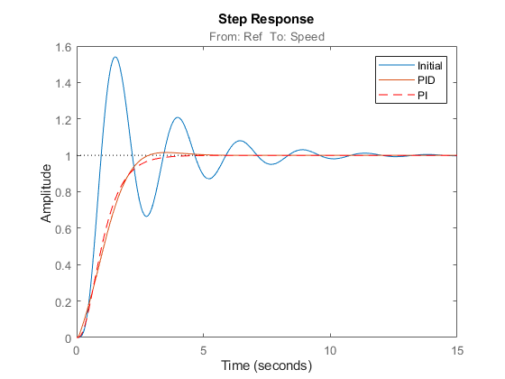
Clearly a PI controller is sufficient for this application.
See Also
systune (slTuner) | slTuner | TuningGoal.Tracking