Troubleshoot Linearization Results in Model Linearizer
This example shows how to interactively debug the linearization of a Simulink® model using the Linearization Advisor within the Model Linearizer app. You can also troubleshoot linearization results programmatically. For more information, see Troubleshoot Linearization Results at Command Line.
Open Model
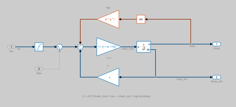
This example using a pendulum Simulink model to demonstrate linearization troubleshooting.
Open the model.
openExample("scdpendulum")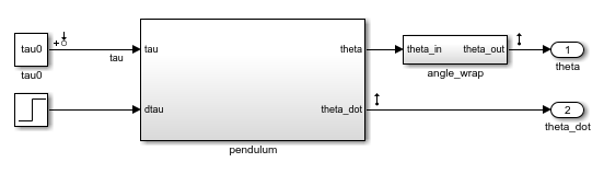
The initial condition for the pendulum angle is 90 degrees counterclockwise from the upright unstable equilibrium of 0 degrees. The initial condition for the pendulum angular velocity is 0 deg/s. The nominal torque to maintain this state is –49.05 N m. This configuration is saved as the model initial condition.
Open Model Linearizer and Linearize Model
To open Model Linearizer, in the Simulink model window, on the Apps tab, click Model Linearizer.
To linearize the model at the model initial condition, in Model Linearizer, on the Linear Analysis tab, click Bode. The software linearizes the model and plots its frequency response.
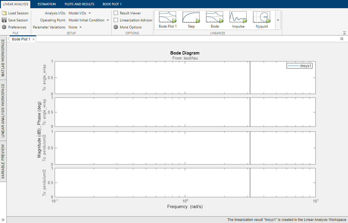
The Bode plot shows that the system linearizes to zero such that the torque has no effect on the angle or angular velocity. You can explore why this is the case using the Linearization Advisor.
Linearize Model with Advisor Enabled
To relinearize the model and generate an advisor, select Linearization Advisor, and click Bode Plot 1.
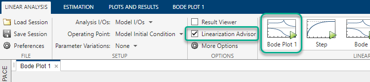
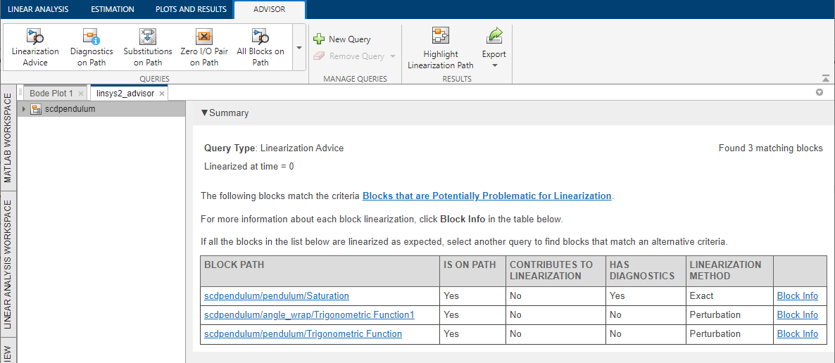
The software linearizes the model, creates the linsys2_advisor document, and opens the Advisor tab.
Highlight Linearization Path
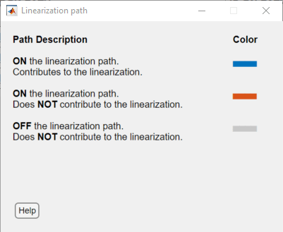
To show the linearization path for the current linearization, on the Advisor tab, click Highlight Linearization Path. In the Simulink model, the blocks highlighted in:
Blue numerically influence the model linearization.
Red are on the linearization path but do not influence the model linearization for the current operating point and block parameters.
For convenience, only the blocks underneath the pendulum subsystem are shown.
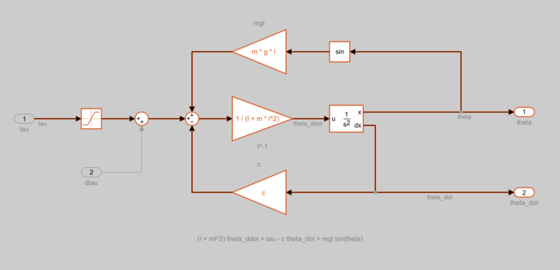
In this case, since the model linearized to zero, there are no blocks that contribute to the linearization.
Investigate Potentially Problematic Blocks Using Advisor
The linsys2_advisor document shows a table listing blocks that may be problematic for the linearization. To view more information about a specific block linearization, in the corresponding row of the table, click Block Info.
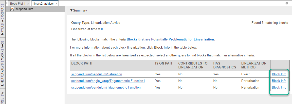
In this case, three blocks are reported by the advisor, a Saturation block and two Trigonometric Function blocks. Investigate the Saturation block first since it has diagnostics. To do so, in the first row of the table, click Block Info.
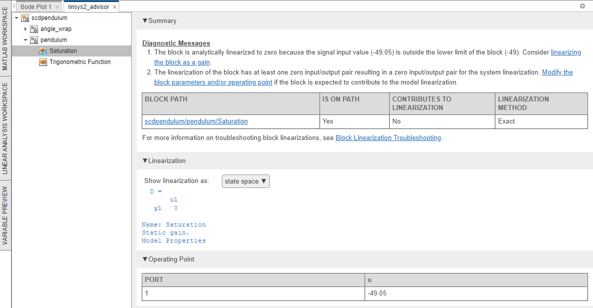
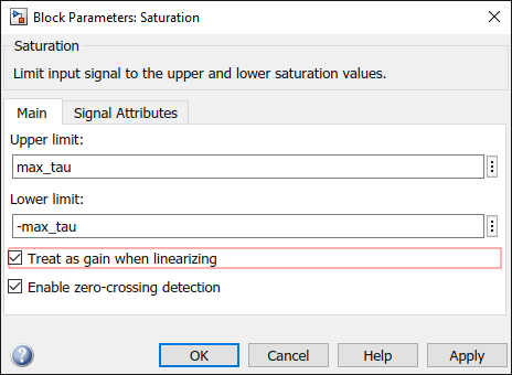
There are two diagnostic messages for the Saturation block. The first message indicates that the block is linearized outside of its lower saturation limit of –49, since the input operating point is –49.05. The message also states the block can be linearized as a gain, which will linearize the block as 1 regardless of the input operating point. To do so, first click linearizing the block as a gain, which highlights the corresponding parameter in the block dialog box. Then, select the Treat as gain when linearizing parameter.
The second message states that the linearization of this block causes the model to linearize to zero. As shown in the Linearization section, the block is linearized to zero. Therefore, modifying the block linearization is a good first step toward obtaining a nonzero model linearization.
Relinearize Model
After setting the Saturation block to be treated as a gain, relinearize the model. For now, ignore the diagnostics for the two Trigonometric Function blocks.
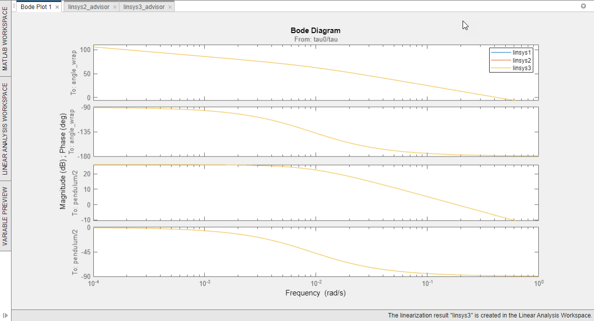
To relinearize the model, on the Linear Analysis tab, click
Bode Plot 1. The Bode Plot 1 document
updates, showing the nonzero response of linsys3.
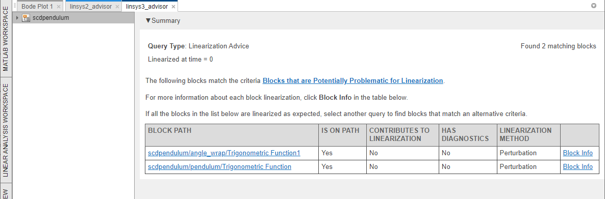
In the corresponding linsys_advisor3 document, the Saturation block is no longer listed. However, the two Trigonometric Function blocks are still shown.
Highlight the linearization path.
Most of the blocks are now contributing to the model linearization, except for the paths going through the listed Trigonometric Function blocks.
To understand why these blocks are not contributing to the linearization, navigate to the blocks from the linsys3_advisor document. For example, click Block Info in the second row of the table.
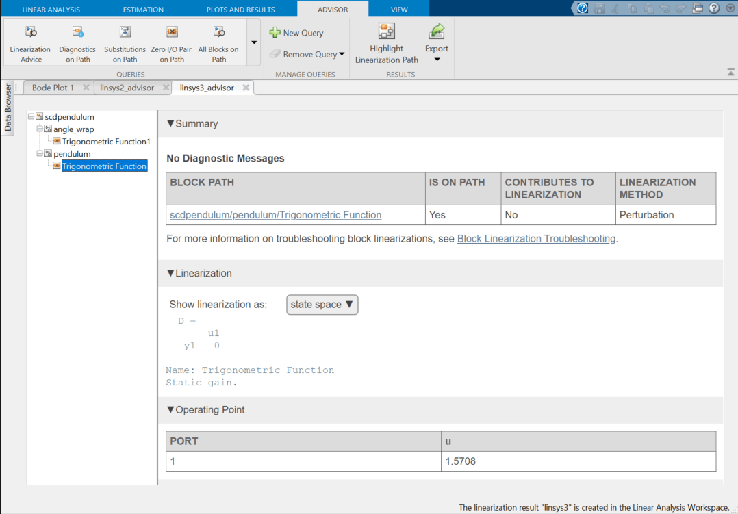
For this Trigonometric Function block, the linearization is zero and the input operating point is π/2 = 1.5708.
You can find the linearization of the block analytically by taking the first
derivative of the sin function with respect to the
inputs.
Therefore, when evaluated at u=π/2 the linearization of the block is zero. The source of the input is the first output of the second-order integrator, which is dependent upon the state theta. Therefore, this block will linearize to zero if θ=π/2 + kπ, where k is an integer. The same condition applies for the other Trigonometric Function in the angle_wrap subsystem.
If these blocks are not expected to linearize to zero, you can modify the operating point state theta, and relinearize the model.
Run Prebuilt Advisor Queries
The Linearization Advisor provides a set of prebuilt queries for filtering block diagnostics. For example, the Linearization Advice query is the default query run when the advisor is first created and includes blocks on the path that meet one of the following criteria:
Have diagnostic messages regarding the block linearization.
Linearize to zero.
Have substituted linearizations.
To run a different prebuilt query, on the Advisor tab, in the Queries gallery, click the query. For example, click Zero I/O Pair on Path.
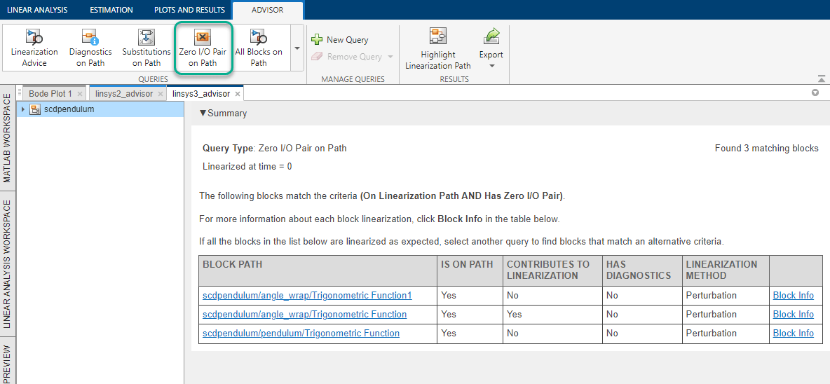
This query returns blocks with linearizations that have output channels that
cannot be reached by any input channel, or input channels that have no influence on
any output channels. For example, the second block in the table is a
Trigonometric Function block configured as
atan2. The first input of this block cannot reach the only
output.
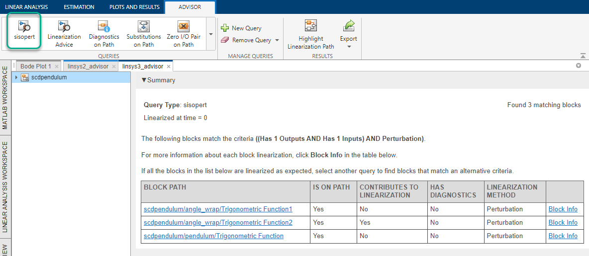
Create and Run Custom Queries
The Linearization Advisor also provides a Query Builder for creating custom queries. You can use these queries to find blocks in your model that match specific criteria. For example, to find all SISO blocks that are numerically perturbed, first open the Query Builder. To do so, on the Advisor tab, click New Query.
In the Query Builder dialog box:
Specify the Query Name as
sisopert.In the drop-down list, select
Has 'Ny' Outputs, and specify1in the Outputs box.To add another component to the query, click Add to Query.
In the second drop-down list, select
Has 'Nu'
                            Inputs
, and specify1in the Inputs box.Click Add to Query.
In the third drop-down list, select
Perturbation.
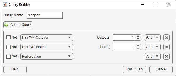
Click Run Query.
The linsys3_advisor document shows the blocks that match the specified query criteria, and the sisopert query is added to the Queries gallery.
For more information on configuring and running custom queries, see Find Blocks in Linearization Results Matching Specific Criteria.
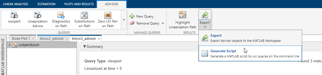
Export Advisor and Generate MATLAB Script
You can also debug model linearizations using the Linearization Advisor command-line functions. To do so, you first export your advisor object to the MATLAB® or generate a MATLAB script to reproduce the analysis from the app.
For more information on debugging linearizations at the command line, see Troubleshoot Linearization Results at Command Line.
Export Advisor
To export your advisor object to the MATLAB workspace, on the Advisor tab, click Export. Then, in the Export Advisors dialog box, select one or more advisors to export. For example, select linsys3_advisor.
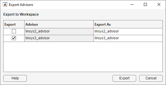
In the Export As column, you can specify a workspace variable name of the exported advisor object.
Click Export.
Generate Script
You can generate a MATLAB script that automates the linearization, extraction of the advisor, generation of custom queries, and running of queries. To generate this script, on the Advisor tab, under Export, select Generate Script.