PID Tuning for Setpoint Tracking vs. Disturbance Rejection
This example uses systune to explore tradeoffs between setpoint tracking and disturbance rejection when tuning PID controllers.
PID Tuning Tradeoffs
When tuning 1-DOF PID controllers, it is often impossible to achieve good tracking and fast disturbance rejection at the same time. Assuming the control bandwidth is fixed, faster disturbance rejection requires more gain inside the bandwidth, which can only be achieved by increasing the slope near the crossover frequency. Because a larger slope means a smaller phase margin, this typically comes at the expense of more overshoot in the response to setpoint changes.
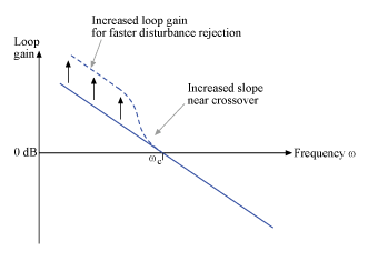
Figure 1: Tradeoff in 1-DOF PID Tuning.
This example uses systune to explore this tradeoff and find the right compromise for your application. You can also use the PID Tuner app to make such a tradeoff. For more information, see Tune PID Controller to Favor Reference Tracking or Disturbance Rejection (PID Tuner).
Tuning Setup
Consider the PID loop of Figure 2 with a load disturbance at the plant input.
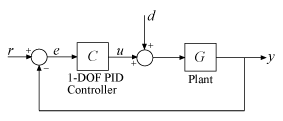
Figure 2: PID Control Loop.
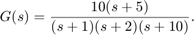
For this example we use the plant model
The target control bandwidth is 10 rad/s. Create a tunable PID controller and fix its derivative filter time constant to  (10 times the bandwidth) so that there are only three gains to tune (proportional, integral, and derivative gains).
G = zpk(-5,[-1 -2 -10],10);
C = tunablePID('C','pid');
C.Tf.Value = 0.01;  C.Tf.Free = false;  % fix Tf=0.01
Construct a tunable model T0 of the closed-loop transfer from r to y. Use an "analysis point" block to mark the location u where the disturbance enters.
LS = AnalysisPoint('u');
T0 = feedback(G*LS*C,1);
T0.u = 'r'; T0.y = 'y';
The gain of the open-loop response  is a key indicator of the feedback loop behavior. The open-loop gain should be high (greater than one) inside the control bandwidth to ensure good disturbance rejection, and should be low (less than one) outside the control bandwidth to be insensitive to measurement noise and unmodeled plant dynamics. Accordingly, use three requirements to express the control objectives:
"Tracking" requirement to specify a response time of about 0.2 seconds to step changes in
r"MaxLoopGain" requirement to force a roll-off of -20 dB/decade past the crossover frequency 10 rad/s
"MinLoopGain" requirement to adjust the integral gain at frequencies below 0.1 rad/s.
s = tf('s');
wc = 10; % target crossover frequency

% Tracking
R1 = TuningGoal.Tracking('r','y',2/wc);

% Bandwidth and roll-off
R2 = TuningGoal.MaxLoopGain('u',wc/s);

% Disturbance rejection
R3 = TuningGoal.MinLoopGain('u',wc/s);
R3.Focus = [0 0.1];
Tuning of 1-DOF PID Controller
Use systune to tune the PID gains to meet these requirements. Treat the bandwidth and disturbance rejection goals as hard constraints and optimize tracking subject to these constraints.
T1 = systune(T0,R1,[R2 R3]);
Final: Soft = 1.12, Hard = 0.9998, Iterations = 158
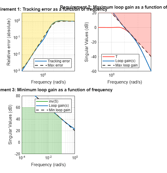
Verify that all three requirements are nearly met. The blue curves are the achieved values and the yellow patches highlight regions where the requirements are violated.
figure('Position',[100,100,560,580])
viewGoal([R1 R2 R3],T1)
Tracking vs. Rejection
To gain insight into the tradeoff between tracking and disturbance rejection, increase the minimum loop gain in the frequency band [0,0.1] rad/s by a factor  . Re-tune the PID gains for the values
  .
.
% Increase loop gain by factor 2
alpha = 2;
R3.MinGain = alpha*wc/s;
T2 = systune(T0,R1,[R2 R3]);
Final: Soft = 1.17, Hard = 0.99954, Iterations = 115
% Increase loop gain by factor 4
alpha = 4;
R3.MinGain = alpha*wc/s;
T3 = systune(T0,R1,[R2 R3]);
Final: Soft = 1.25, Hard = 0.99994, Iterations = 166
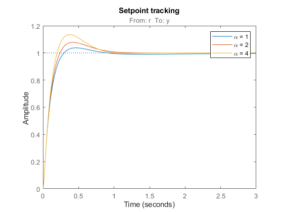
Compare the responses to a step command r and to a step disturbance d entering at the plant input u.
figure, step(T1,T2,T3,3)
title('Setpoint tracking')
legend('\alpha = 1','\alpha = 2','\alpha = 4')
% Compute closed-loop transfer from u to y
D1 = getIOTransfer(T1,'u','y');
D2 = getIOTransfer(T2,'u','y');
D3 = getIOTransfer(T3,'u','y');
step(D1,D2,D3,10)
title('Disturbance rejection')
legend('\alpha = 1','\alpha = 2','\alpha = 4')
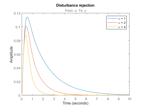
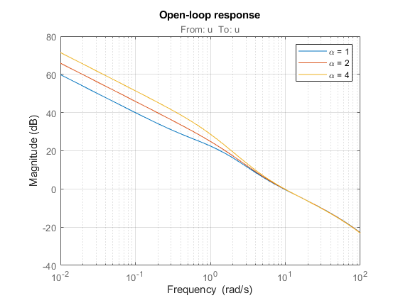
Note how disturbance rejection improves as alpha increases, but at the expense of increased overshoot in setpoint tracking. Plot the open-loop responses for the three designs, and note how the slope before crossover (0dB) increases with alpha.
L1 = getLoopTransfer(T1,'u');
L2 = getLoopTransfer(T2,'u');
L3 = getLoopTransfer(T3,'u');
bodemag(L1,L2,L3,{1e-2,1e2}), grid
title('Open-loop response')
legend('\alpha = 1','\alpha = 2','\alpha = 4')
Which design is most suitable depends on the primary purpose of the feedback loop you are tuning.
Tuning of 2-DOF PID Controller
If you cannot compromise tracking to improve disturbance rejection, consider using a 2-DOF architecture instead. A 2-DOF PID controller is capable of fast disturbance rejection without significant increase of overshoot in setpoint tracking.
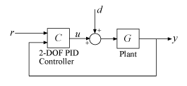
Figure 3: 2-DOF PID Control Loop.
Use the tunablePID2 object to parameterize the 2-DOF PID controller and construct a tunable model T0 of the closed-loop system in Figure 3.
C = tunablePID2('C','pid');
C.Tf.Value = 0.01;  C.Tf.Free = false;  % fix Tf=0.01

T0 = feedback(G*LS*C,1,2,1,+1);
T0 = T0(:,1);
T0.u = 'r';  T0.y = 'y';
Next tune the 2-DOF PI controller for the largest loop gain tried earlier ( ).
).
% Minimum loop gain inside bandwidth (for disturbance rejection)
alpha = 4;
R3.MinGain = alpha*wc/s;

% Tune 2-DOF PI controller
T4 = systune(T0,R1,[R2 R3]);
Final: Soft = 1.09, Hard = 0.86236, Iterations = 72
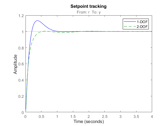
Compare the setpoint tracking and disturbance rejection properties of the 1-DOF and 2-DOF designs for .
clf, step(T3,'b',T4,'g--',4)
title('Setpoint tracking')
legend('1-DOF','2-DOF')
D4 = getIOTransfer(T4,'u','y');
step(D3,'b',D4,'g--',4)
title('Disturbance rejection')
legend('1-DOF','2-DOF')
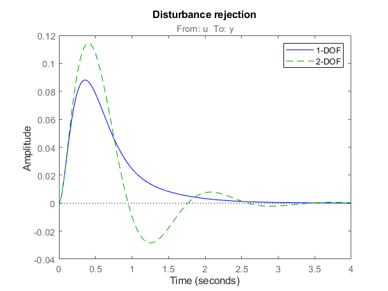
The responses to a step disturbance are similar but the 2-DOF controller eliminates the overshoot in the response to a setpoint change. You can use showTunable to compare the tuned gains in the 1-DOF and 2-DOF controllers.
showTunable(T3) % 1-DOF PI
C =

             1            s
  Kp + Ki * --- + Kd * --------
             s          Tf*s+1

  with Kp = 9.51, Ki = 14.9, Kd = 0.89, Tf = 0.01

Name: C
Continuous-time PIDF controller in parallel form.
showTunable(T4) % 2-DOF PI
C =

                       1                s
  u = Kp (b*r-y) + Ki --- (r-y) + Kd -------- (c*r-y)
                       s              Tf*s+1

  with Kp = 5.6, Ki = 22.1, Kd = 0.848, Tf = 0.01, b = 0.641, c = 1.32

Name: C
Continuous-time 2-DOF PIDF controller in parallel form.