Measure Three-Phase Electric Circuit Impedance Using Sinestream Signal Generator Block

Since R2024b

This example shows how to use the Sinestream Signal Generator block to inject a sinestream input signal that measures the three-phase electric circuit impedance through an offline frequency response estimation experiment. In practice, you can use this approach to perform the experiment in real-time against a physical plant. In this example, you perform the experiment on a plant modeled in Simulink®.

Examine Model

This example uses a Simulink® model that contains a three-phase circuit as the plant model. The model is preconfigured with a Sinestream Signal Generator block that injects a perturbation signal at the plant input. The model also collects the circuit response data, which you can use for offline frequency response estimation.

Open the model.

mdl = "SineSigGenZPowerGridPorts.slx";
open_system(mdl)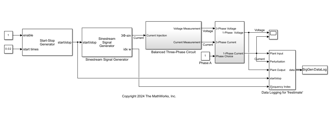

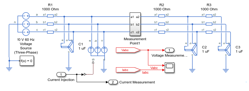
Electric Circuit

The electric circuit plant model is a three-phase passive AC network. There is one point for current injection using a Controlled Current Source (Three-Phase) block. There are two measurement subsystems at the source and the network side. The three-phase voltage and current measurements are routed to data logging for impedance measurements.

Signal Parameter Settings

The Sinestream Signal Generator block is parameterized to generate a sinestream signal at 20 frequency points between 10 rad/s and 10,000 rad/s, all with amplitudes of 10. In addition, there are three periods of signal for each frequency point. The Signal Length section of the block parameters displays the required experiment length based on the current block parameter settings. To ensure a comprehensive experiment, you must configure the Start-Stop Generator block such that the signal injects for at least that long.

The Advanced Settings section contains parameters that you can use to configure the sinestream signal type and form. You can choose to generate sine signals, cosine signals, or both using the Waveform Type parameter. You can also use the Phase Shift parameter to configure a consistent phase shift in the generated signals.

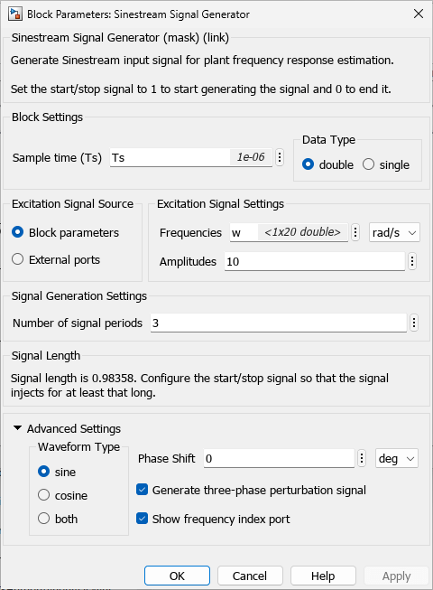
In this example, the Show frequency index port parameter is enabled. This option enables the output port idx w. During simulation, the signal at this port shows the corresponding index of the generated frequency component. A staircase signal helps the post-processing of the logged experiment data. This signal generates a Ready signal similar to the signal output by the Frequency Response Estimator block.

The Generate three-phase perturbation signal parameter allows you to generate balanced three-phase perturbation signals. The generated signal is balanced because the summation of these three-phase signals always equals zero. You can use these signals to analyze three-phase alternating current (AC) electric circuits.

Collect Experiment Data

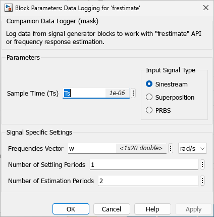
The Data Logging for 'frestimate' subsystem collects experiment data at the point of signal injection, on the source side, and on the network side in the data objects SigGenDataLog, SigGenDataLogSource, and SigGenDataLogNetwork, respectively. The subsystem logs the Ready, Perturbation, PlantInput, and PlantOutput signals in each data object. Inside the Data Logging for 'frestimate' subsystems, the Subtract Nominal Values subsystem removes the nominal values from the logged input and output signals.

Simulate the model. The model injects the generated sinestream perturbation signals into the electric circuit and collects the measurements.

sim(mdl)

The model collects the data in the format compatible for offline frequency response estimation.

SigGenDataLogBus
SigGenDataLogNetwork
SigGenDataLogSource

The Ready field is a timeseries signal that contains a logical signal that indicates which time steps contain the data to use for the estimation. For a sinestream signal, this field indicates the settling periods, which are the perturbation periods for the estimation to discard. Perturbation contains the sinestream perturbation applied to the plant. The PlantInput and PlantOutput timeseries signals contain the input and output signals of the plant.

Calculate Analytical Impedance

Based on the circuit model, you can express the impedance as a continuous transfer function. By discretizing the transfer function, you can use it as a reference for the offline frequency response estimation result.

Define the analytical impedance at the bus signal injection.

analyticalTFbus = tf([R^3*C^2 3*R^2*C R],[R^3*C^3 5*R^2*C^2 6*R*C 1])
TFdbus = c2d(analyticalTFbus,Ts);
analyticalFRDbus = frd(TFdbus,w,"rad/s"); % convert to frd object

Define the analytical impedance on the network side.

analyticalTFnetwork = tf([R^2*C^2 3*R*C 1],[R*C^2 2*C 0])
TFdnetwork = c2d(analyticalTFnetwork,Ts,'tustin');
analyticalFRDnetwork = frd(TFdnetwork,w,"rad/s"); % convert to frd object

Define the analytical impedance on the source side.

analyticalTFsource = tf([R],[R*C 1])
TFdsource = c2d(analyticalTFsource,Ts,'tustin');
analyticalFRDsource = frd(TFdsource,w,"rad/s"); % convert to frd object

Estimate Frequency Response

To perform the frequency response estimation offline, use the collected data with the frestimate function.

Use the logged data structures and the specified frequencies as inputs to the frestimate function. frestimate processes the logged data to obtain a frequency response data model that contains the estimated responses at the specified frequencies. The logged data objects are SigGenDataLogBus, SigGenDataLogNetwork, and SigGenDataLogSource.

sys_estim_bus = frestimate(SigGenDataLogBus,w,"rad/s");
size(sys_estim_bus)
sys_estim_network = frestimate(SigGenDataLogNetwork,w,"rad/s");
size(sys_estim_network)
sys_estim_source = frestimate(SigGenDataLogSource,w,"rad/s");
size(sys_estim_source)

Examine Estimated Frequency Response

Compare the frequency response estimation result with the derived analytical transfer functions.

ZdataOffline_bus = reshape(sys_estim_bus.ResponseData,[1,Nf]);
ZdataOffline_network = reshape(sys_estim_network.ResponseData,[1,Nf]);
ZdataOffline_source = reshape(sys_estim_source.ResponseData,[1,Nf]);
ZdataAnalyticalbus = reshape(analyticalFRDbus.ResponseData,[1,Nf]);
ZdataAnalyticalnetwork = reshape(analyticalFRDnetwork.ResponseData,[1,Nf]);
ZdataAnalyticalsource = reshape(analyticalFRDsource.ResponseData,[1,Nf]);
figure;
subplot(2,1,1);
semilogx(w/(2*pi),abs(ZdataOffline_bus),'b*'); 
hold on
semilogx(w/(2*pi),abs(ZdataAnalyticalbus),'ro');
title('Impedance Measurement at Bus of Injection');
ylabel('Amplitude [Ohm]');
legend('Offline FRE','Analytical');
grid on;
subplot(2,1,2);
semilogx(w/(2*pi),angle(ZdataOffline_bus)*180/pi,'b*');
hold on
semilogx(w/(2*pi),angle(ZdataAnalyticalbus)*180/pi, 'ro');
xlabel('Frequency [Hz]');
ylabel('theta [deg]');
grid on;
figure;
subplot(2,1,1);
semilogx(w/(2*pi),abs(ZdataOffline_network),'b*'); 
hold on
semilogx(w/(2*pi),abs(ZdataAnalyticalnetwork),'ro');
title('Impedance Measurement of Network');
ylabel('Amplitude [Ohm]');
legend('Offline FRE','Analytical TF');
grid on;
subplot(2,1,2);
semilogx(w/(2*pi),angle(ZdataOffline_network)*180/pi,'b*');
hold on
semilogx(w/(2*pi),angle(ZdataAnalyticalnetwork)*180/pi, 'ro');
xlabel('Frequency [Hz]');
ylabel('theta [deg]');
grid on;
figure;
subplot(2,1,1);
semilogx(w/(2*pi),abs(ZdataOffline_source),'b*'); 
hold on
semilogx(w/(2*pi),abs(ZdataAnalyticalsource),'ro');
title('Impedance Measurement of Source');
ylabel('Amplitude [Ohm]');
legend('Offline FRE','Analytical TF');
grid on;
subplot(2,1,2);
semilogx(w/(2*pi),angle(ZdataOffline_source)*180/pi,'b*');
hold on
semilogx(w/(2*pi),angle(ZdataAnalyticalsource)*180/pi, 'ro');
xlabel('Frequency [Hz]');
ylabel('theta [deg]');
grid on;

The impedance measurement matches the analytical results from the derived transfer functions.

You can also use the Sinestream Signal Generator block to conduct impedance measurement in a single-phase circuit. Additionally, you can also conduct multiple frequency response estimation experiments over various operating conditions.