Validate Linearization in Frequency Domain at Command Line

This example shows how to validate a block-by-block analytical linearization result using frequency response estimation. To run this example, you need Aerospace Blockset™ software.

Linearize Model

Open the Simulink® model for the lightweight airplane. For more information on this model, see Lightweight Airplane Design (Aerospace Blockset).

mdl = 'scdskyhogg';
open_system(mdl)

You can linearize the lightweight airplane model from the altitude command signal, AltCmd, to the sensed height, h_sensed. These linear analysis points are already specified in the model.

io = getlinio(mdl)

2x1 vector of Linearization IOs: 
--------------------------
1. Linearization input perturbation located at the following signal:
- Block: scdskyhogg/Pilot/Add
- Port: 1
- Signal Name: AltCmd
2. Linearization output measurement located at the following signal:
- Block: scdskyhogg/Vehicle System Model/Avionics/Autopilot/Bus Selector1
- Port: 1
- Signal Name: <h_sensed>

Linearize the model using the linearize function. The model is preconfigured to use an operating point obtained using a simulation snapshot at t = 75.

sys = linearize(mdl,io);
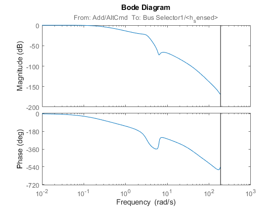
bode(sys)

Estimate Frequency Response

To determine whether the linearization results properly capture characteristics of the nonlinear model, such as the anti-resonance around 6.28 rad/s, you can validate the linearization result using frestimate.

Create a sinestream input signal. Use the linearization result as an input argument to automatically set various parameters of the sinestream input signal, such as the set of frequencies and the number of periods for each frequency, based on the linear system.

in = frest.Sinestream(sys);
in.Amplitude = 0.5

 
The sinestream input signal:
 
      Frequency           : [0.0034142;0.0054345;0.0086502;0.013768 ...] (rad/s)
      Amplitude           : 0.5
      SamplesPerPeriod    : [110417;69370;43582;27381 ...]
      NumPeriods          : [4;4;4;4 ...]
      RampPeriods         : 0
      FreqUnits (rad/s,Hz): rad/s
      SettlingPeriods     : [1;1;1;1 ...]
      ApplyFilteringInFRESTIMATE (on/off)    : on
      SimulationOrder (Sequential/OneAtATime): Sequential
 

The software selects 25 frequencies at which to compute the response. These frequencies vary between 0.0034 rad/s and 14.5 rad/s. The frequencies that are automatically selected focus on where interesting dynamics occur (such as the anti-resonance at 6.28 rad/s). The number of periods that it takes for the system to reach steady state is estimated for each of these frequencies and varies between 1 period (for 0.0034 rad/s) and 188 periods (for 14.5 rad/s).

Estimate the frequency response using this input signal. frestimate simulates the model with the input signal, which can take a long time in a normal simulation model. To speed up the simulation, configure the model to use rapid accelerator mode.

set_param(mdl,'SimulationMode','rapid');

Using rapid accelerator mode can significantly increase the speed of the simulation. The actual speed improvement depends on your computer configuration.

To run the frequency response estimation use the following command.

sysest = frestimate(mdl,in,io);

For this example, you can load the estimation result from a MAT-file.

load scdskyhogg_frestresults.mat;

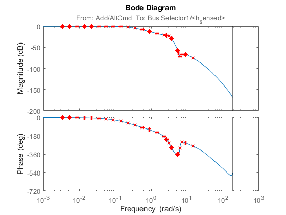
Compare the analytical linearization result against the frequency response data from frestimate. The frequency response data and analytical linearization result match well, validating that anti-resonance between the frequencies 1 and 10 rad/s does exist in the actual nonlinear airplane model.

bode(sys,sysest,'r*')

Close the model.

bdclose('scdskyhogg')