Fanno Flow Gas Pipe Validation

The Fanno flow model is an analytical solution of an adiabatic (perfectly insulated) compressible perfect gas flow through a constant area pipe with friction. This example shows a comparison and validation of the Simscape™ Pipe (G) block against the Fanno flow model. While you typically need empirical data to validate a block over a range of scenarios, it may still be useful to perform limited validation against analytical models for specific scenarios. This is because the theory and derivation behind the analytical model may provide more insight into where the block works well and how to address limitations. The comparison shows that, for short to moderate pipe lengths, the Simscape pipe model agrees well with the Fanno flow model. For long pipe lengths, a segmented pipe model agrees well with the Fanno flow model.

Model Data

% Load models
model = "FannoFlowGasPipeValidation";
load_system(model)
modelSegmented = "FannoFlowGasPipeValidationSegmented";
load_system(modelSegmented)

Before opening the Simscape model, define the data for the Fanno flow problem and plot the analytical solution:

% Pipe geometry
D = 0.1;           % m   Diameter
A = pi*D^2/4;      % m^2 Cross-sectional area
roughness = 15e-6; % m   Surface roughness

% Perfect gas properties
R = 287;    % J/(kg*K) Specific gas constant
cp = 1e3;   % J/(kg*K) Specific heat at constant pressure
mu = 18e-6; % Pa*s     Dynamic viscosity

% Inlet conditions
p1 = 2e5; % Pa         Inlet static pressure
T1 = 300; % K          Inlet static temperature
mdot = 1; % kg/(s*m^2) Mass flow rate

Compute additional fluid properties at the inlet:

% Inlet density [kg/m3]
rho1 = p1/(R*T1)

rho1 = 2.3229

 % Ratio of specific heats
gamma = cp/(cp - R)

gamma = 1.4025

% Speed of sound at inlet [m/s]
a1 = sqrt(gamma*R*T1)

a1 = 347.5016

% Inlet Mach number
M1 = mdot/(rho1*a1*A)

M1 = 0.1577

The Fanno flow model assumes a constant friction factor over the length of the pipe. Like the Pipe (G) block, calculate the Darcy friction factor using the Haaland correlation:

% Reynolds number
Re = (mdot*D)/(mu*A)

Re = 7.0736e+05

% Darcy friction factor
fD = 1 / (-1.8 * log10(6.9/Re + (roughness/(3.7*D))^1.11))^2

fD = 0.0144

Analytical Fanno Flow Model

The assumption of constant area adiabatic flow, constant friction factor, and perfect gas results in the following steady-state spatial differential equation:

$$\frac{{\mathit{f}}_{\mathit{D}}\mathrm{dx}}{{\mathit{D}}_{\mathit{h}}}=\frac{\left(1-{\mathit{M}}^2\right){\mathrm{dM}}^2}{\gamma {\mathit{M}}^4\left(1+\frac{\gamma -1}{2}{\mathit{M}}^2\right)}$$,

where $\mathit{x}$ is the distance along the pipe, $\mathit{M}$ is the Mach number, $\gamma$ is the ratio of specific heats, ${\mathit{D}}_{\mathit{h}}$ is the hydraulic diameter, and ${\mathit{f}}_{\mathit{D}}$ is the Darcy friction factor.

Integrating this equation over an arbitrary length of pipe produces the analytical Fanno flow relations that relate the fluid states at the two ends of this length of pipe. As the length is arbitrary, the Fanno flow relations actually hold for the fluid states at any two locations along the pipe.

Fanno Flow Relations

As the fluid travels down the pipe, changes in the fluid states due to friction cause the Mach number to tend toward $\mathit{M}=1$ regardless of the starting Mach number. This is the sonic (i.e., choked) condition, and the fluid properties at this location are denoted with an asterisk. It is common to simplify the Fanno flow relations such that one end of the pipe is fixed at the sonic condition.

Let the sonic length ${\mathit{L}}^{*}$ be the length of pipe needed to reach the sonic condition starting from any location along with the pipe with Mach number $\mathit{M}$. The Fanno parameter based on the sonic length is

$$\frac{{\mathit{f}}_{\mathit{D}}{\mathit{L}}^{*}}{{\mathit{D}}_{\mathit{h}}}=\frac{1-{\mathit{M}}^2}{\gamma {\mathit{M}}^2}+\frac{\gamma +1}{2\gamma }\ln \left(\frac{\frac{\gamma +1}{2}{\mathit{M}}^2}{1+\frac{\gamma -1}{2}{\mathit{M}}^2}\right)$$.

The ratio of pressure $\mathit{p}$ at a location with Mach number $\mathit{M}$ to the sonic pressure ${\mathit{p}}^{*}$ is

$$\frac{\mathit{p}}{{\mathit{p}}^{*}}=\frac{1}{\mathit{M}}\sqrt{\frac{\frac{\gamma +1}{2}}{1+\frac{\gamma -1}{2}{\mathit{M}}^2}}$$.

The ratio of temperature $\mathit{T}$ at a location with Mach number $\mathit{M}$ to the sonic temperature ${\mathit{T}}^{*}$ is

$$\frac{\mathit{T}}{{\mathit{T}}^{*}}=\frac{\frac{\gamma +1}{2}}{1+\frac{\gamma -1}{2}{\mathit{M}}^2}$$.

The ratio of the change in specific entropy from a location with Mach number $\mathit{M}$ to the sonic condition $\mathit{s}-{\mathit{s}}^{*}$ to the specific gas constant $\mathit{R}$ is

$$\frac{\mathit{s}-{\mathit{s}}^{*}}{\mathit{R}}=\ln \left[{\mathit{M}\left(\frac{\frac{\gamma +1}{2}}{1+\frac{\gamma -1}{2}{\mathit{M}}^2}\right)}^{\frac{\gamma +1}{2\left(\gamma -1\right)}}\right]$$.

% Fanno flow relations as anonymous functions of Mach number
M_fcn = @(M) 1 + (gamma-1)/2 * M.^2;
p_ratio = @(M) sqrt((gamma+1)/2 ./ M_fcn(M)) ./ M;
T_ratio = @(M) (gamma+1)/2 ./ M_fcn(M);
delta_s_R = @(M) log(M .* ((gamma+1)/2 ./ M_fcn(M)).^((gamma+1)/2/(gamma-1)));
fanno = @(M) (1 - M.^2)./(gamma*M.^2) + (gamma+1)/(2*gamma) * log((gamma+1)/2 .* M.^2 ./ M_fcn(M));

Sonic Condition

Using the specified inlet conditions and the Fanno flow relations, calculate the sonic conditions that a sufficiently long pipe will reach:

% Sonic outlet pressure [Pa]
p_star = p1/p_ratio(M1)

p_star = 2.8855e+04

% Sonic outlet temperature [K]
T_star = T1/T_ratio(M1)

T_star = 250.9878

% Sonic outlet specific enthalpy [J/kg]
h_star = cp*T_star %#ok<NASGU>

h_star = 2.5099e+05

% Sonic outlet density [kg/m^3]
rho_star = p_star/(R*T_star)

rho_star = 0.4006

% Pipe length to reach sonic outlet condition from inlet condition [m]
L_star = fanno(M1) * D / fD

L_star = 173.6802

Given the relatively low inlet Mach number of about 0.16, it takes a long pipe to reach the sonic condition. The required length to diameter ratio is

L_star/D

ans = 1.7368e+03

Plot Fanno Line

By varying the Mach number, the Fanno flow relations trace a locus of points in an enthalpy-entropy (H-S) diagram, known as the Fanno line. Any point on the line represents the fluid states at a location along the pipe for the given flow.

M_range = [0.15 3];
figure
fplot(@(M) delta_s_R(M)*R, @(M) T_ratio(M)*T_star*cp, M_range, LineWidth = 1)
grid on
xlabel("Specific Entropy [J/(kg*K)]")
ylabel("Specific Enthalpy [J/kg]")
title("Fanno Line")

As fluid flows along the pipe, entropy is generated due to friction. Therefore, the fluid state moves to the right along either the top curve or the bottom curve of the Fanno line. The right-most point on the Fanno line is the sonic condition with $\mathit{M}=1$. The top curve represents fluid states along the pipe starting from a subsonic ($\mathit{M}<1$) inlet condition moving toward the sonic condition. The bottom curve represents fluid states along the pipe starting from a supersonic ($\mathit{M}>1$) inlet condition moving toward the sonic condition.

The various ratios relative to the sonic condition can also be plotted as a function of Mach number. The plot shows a large change in pressure and density to go from an inlet Mach number of around 0.16 to the sonic condition.

figure
fplot(fanno, M_range, "k", LineWidth = 1)
hold on
set(gca, "ColorOrderIndex", 1)
fplot(p_ratio, M_range, LineWidth = 1)
fplot(T_ratio, M_range, LineWidth = 1)
fplot(@(M) p_ratio(M)./T_ratio(M), M_range, LineWidth = 1)
hold off
grid on
ylim([0 5])
xlabel("Mach Number")
ylabel("Ratios Relative to Sonic Condition")
title("Fanno Flow Relation Curves")
legend("f_DL^*/D_h", "p/p^*", "T/T^*", "\rho/\rho^*", "Location", "best")

Simscape Pipe Model

The Simscape model consists of an upstream reservoir where the inlet conditions are specified, a pipe, a flow rate source where the mass flow rate is specified, and a downstream reservoir. The flow rate source is at the downstream end of the pipe because the pipe inlet must be fixed at the upstream reservoir conditions to match the Fanno flow problem setup. You can compare sensor measurements at the pipe outlet against the analytical Fanno flow model.

open_system(model)

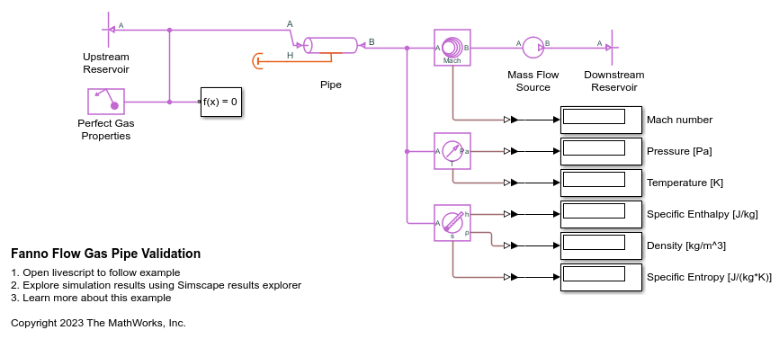
A few of items to note about the Simscape model: First, in the Perfect Gas Properties block, the reference specific enthalpy is 0 J/kg at a reference temperature of 0 K to match the convention in the Fanno line plot. An alternative is to shift the y-axis of the Fanno line plot.

Second, in the Thermodynamic Properties Sensor (G) block, the reference specific entropy is 0 J/(kg*K) at the sonic condition to match the convention in the Fanno line plot. An alternative is to shift the x-axis of the Fanno line plot.

Third, the Simscape gas library models subsonic flow up to the sonic condition. It does not model supersonic flow. Therefore, the comparison is for the subsonic (top) portion of the Fanno line only.

Solve Fanno Flow Model

Given the inlet conditions and a set of pipe lengths from 1 m to 173 m (almost the sonic length), solve the Fanno flow relations to calculate the outlet conditions of the pipe:

% Set of pipe lengths [m]
L_list = [1 76 119 143 156 164 168 171 172 173];

M2 = zeros(size(L_list)); % Outlet Mach number
p2 = zeros(size(L_list)); % Outlet pressure
T2 = zeros(size(L_list)); % Outlet temperature
h2 = zeros(size(L_list)); % Outlet specific enthalpy
rho2 = zeros(size(L_list)); % Outlet density
delta_s2 = zeros(size(L_list)); % Change in specific entropy from inlet to outlet

for i = 1 : numel(L_list)
    L = L_list(i);
    % Solve for outlet Mach number for pipe length L
    M2(i) = fzero(@(M2) fanno(M1) - fanno(M2) - L*fD/D, [M1 1]);
    % Compute outlet conditions from outlet Mach number
    p2(i) = p_ratio(M2(i))*p_star;
    T2(i) = T_ratio(M2(i))*T_star;
    h2(i) = cp*T2(i);
    rho2(i) = p_ratio(M2(i))/T_ratio(M2(i))*rho_star;
    delta_s2(i) = delta_s_R(M2(i))*R;
end

Simulate Simscape Model

Simulate the Simscape model for the same set of pipe lengths and measure the outlet conditions. The pipe length parameter in the pipe block is already configured to Run-time. Turn on Fast Restart mode to simulate each pipe length without recompiling the model.

M2_sim = zeros(size(L_list)); % Outlet Mach number
p2_sim = zeros(size(L_list)); % Outlet pressure
T2_sim = zeros(size(L_list)); % Outlet temperature
h2_sim = zeros(size(L_list)); % Outlet specific enthalpy
rho2_sim = zeros(size(L_list)); % Outlet density
delta_s2_sim = zeros(size(L_list)); % Change in specific entropy from inlet to outlet

set_param(model, "FastRestart", "on")
for i = 1 : numel(L_list)
    L = L_list(i);
    % Simulate model
    out = sim(model);
    % Retrieve simulation results from logged data at last time step
    tmp = out.simlog_FannoFlowGasPipeValidation.Mach_Number_Sensor_G.Mach.series.values("1");
    M2_sim(i) = tmp(end);
    tmp = out.simlog_FannoFlowGasPipeValidation.Pressure_Temperature_Sensor_G.Pa.series.values("Pa");
    p2_sim(i) = tmp(end);
    tmp = out.simlog_FannoFlowGasPipeValidation.Pressure_Temperature_Sensor_G.T.series.values("K");
    T2_sim(i) = tmp(end);
    tmp = out.simlog_FannoFlowGasPipeValidation.Thermodynamic_Properties_Sensor_G.H.series.values("J/kg");
    h2_sim(i) = tmp(end);
    tmp = out.simlog_FannoFlowGasPipeValidation.Thermodynamic_Properties_Sensor_G.RHO.series.values("kg/m^3");
    rho2_sim(i) = tmp(end);
    tmp = out.simlog_FannoFlowGasPipeValidation.Thermodynamic_Properties_Sensor_G.S.series.values("J/(kg*K)");
    delta_s2_sim(i) = tmp(end);
end
set_param(model, "FastRestart", "off")

Plot Comparison

The following plot shows markers for the pipe outlet conditions calculated with Fanno flow model and the Simscape pipe block overlaid on the Fanno line. Each marker represents a different pipe length from the same specified inlet conditions. The left-most marker corresponds to 1 m and the right-most marker corresponds to 173 m.

figure
fplot(@(M) delta_s_R(M)*R, @(M) T_ratio(M)*T_star*cp, M_range, LineWidth = 1)
hold on
set(gca, "ColorOrderIndex", 1)
plot(delta_s2, h2, "x", LineWidth = 1)
set(gca, "ColorOrderIndex", 1)
plot(delta_s2_sim, h2_sim, "s", LineWidth = 1)
hold off
grid on
xlabel("Specific Entropy [J/(kg*K)]")
ylabel("Specific Enthalpy [J/kg]")
title("Outlet Conditions Overlaid on Fanno Line")
legend("", "Fanno Model", "Pipe Block", "Location", "best")

The plot shows good agreement for shorter lengths but a discrepancy for longer lengths. All of the markers from the Simscape simulation lie on the Fanno line locus, but the markers to the right are shifted along the Fanno line relative to the Fanno flow model markers. Since the Fanno line locus corresponds to different Mach numbers, this suggests that the Simscape simulation calculated lower outlet Mach numbers for long pipe lengths, but the compressible flow fluid properties at those Mach numbers are accurate.

The following plot shows markers for the outlet pressure, temperature, and density at various pipe lengths relative to the sonic values overlaid on the Fanno flow relation curves. The x-axis values for the markers indicate the outlet Mach number at those pipe lengths. As above, all of the markers from the Simscape simulation lie on the Fanno flow relation curves, but the markers at higher outlet Mach numbers (longer pipe lengths) are shifted relative to the Fanno flow model markers.

figure
fplot(fanno, M_range, "k", LineWidth = 1)
hold on
set(gca, "ColorOrderIndex", 1)
fplot(p_ratio, M_range, LineWidth = 1)
fplot(T_ratio, M_range, LineWidth = 1)
fplot(@(M) p_ratio(M)./T_ratio(M), M_range, LineWidth = 1)
set(gca, "ColorOrderIndex", 1)
plot(M2, p2/p_star, "x", LineWidth = 1)
plot(M2, T2/T_star, "x", LineWidth = 1)
plot(M2, rho2/rho_star, "x", LineWidth = 1)
set(gca, "ColorOrderIndex", 1)
plot(M2_sim, p2_sim/p_star, "s", LineWidth = 1)
plot(M2_sim, T2_sim/T_star, "s", LineWidth = 1)
plot(M2_sim, rho2_sim/rho_star, "s", LineWidth = 1)
hold off
grid on
ylim([0 5])
xlabel("Mach Number")
ylabel("Ratios Relative to Sonic Condition")
title("Outlet Conditions Overlaid on Fanno Flow Relation Curves")
legend("f_DL^*/D_h", "", "", "", ...
    "p/p^* Fanno Model", "T/T^* Fanno Model", "\rho/\rho^* Fanno Model", ...
    "p/p^* Pipe Block", "T/T^* Pipe Block", "\rho/\rho^* Pipe Block", "Location", "best")

The discrepancy is that the outlet Mach number from the Simscape model is less than the Fanno flow model at long pipe lengths. The following plot of distance along pipe vs Mach number shows this more clearly. It also shows that the pipe length increases rapidly with Mach number, or, rather, the outlet Mach number does not increase much until the pipe length becomes very long. The discrepancy is small until $\mathit{L}>160$ m, or $\mathit{L}/\mathit{D}>1600$.

figure
fplot(@(M) L_star - fanno(M)*D/fD, M_range, LineWidth = 1)
hold on
set(gca, "ColorOrderIndex", 1)
plot(M2, L_list, "x", LineWidth = 1)
set(gca, "ColorOrderIndex", 1)
plot(M2_sim, L_list, "s", LineWidth = 1)
hold off
grid on
ylim([0 L_star])
xlabel("Mach Number")
ylabel("Distance [m]")
title("Distance Along Pipe vs Mach Number")
legend("", "Fanno Model", "Pipe Block", "Location", "best")

Simscape blocks are lumped parameter models which model the average or aggregate states of a physical component. For example, the pipe block models its internal fluid volume as a single unit and implements the integral form of the conservation equations to determine the aggregate fluid states of that volume. As such, it is less accurate than the analytical Fanno model which incorporates the continuous distribution of fluid properties, but more accurate than a single element of a computational fluid dynamics (CFD) model. This also suggests that dividing a long pipe into multiple pipe blocks in series may improve accuracy.

Segmented Simscape Pipe Model

The pipe block implements the integral mass, momentum, and energy conservation equations to capture the aggregate change in fluid states. However, the momentum conservation equation depends on a pressure loss term, which is related to the friction factor:

$$\Delta {\mathit{p}}_{\mathrm{loss}}=\left(\frac{{\dot{\mathit{m}}}^2}{2\rho {\mathit{A}}^2}\right)\left(\frac{{\mathit{f}}_{\mathit{D}}\mathit{L}}{{\mathit{D}}_{\mathit{h}}}\right)$$.

Because the pipe block computes an average density for the internal fluid volume, this $\Delta {\mathit{p}}_{\mathrm{loss}}$ term will not be accurate if there is a significant variation in density from inlet to outlet. Indeed, from the Fanno flow relations plot, we see that density changes by a factor of around 4 from the inlet to outlet for the longest pipe length. This is why the outlet Mach number from the Simscape model is lower than the Fanno flow model.

One method to improve the accuracy of the Simscape model for long pipe lengths is to divide the pipe into multiple segments. The following Simscape model is the same as before except that the pipe has been divided into 5 segments.

open_system(modelSegmented)

The subsystem consists of 5 pipe blocks, each with length $\mathit{L}/5$.

Simulate Simscape Model

Simulate the model for the same set of pipe lengths and measure the outlet conditions:

M2_seg = zeros(size(L_list)); % Outlet Mach number
p2_seg = zeros(size(L_list)); % Outlet pressure
T2_seg = zeros(size(L_list)); % Outlet temperature
h2_seg = zeros(size(L_list)); % Outlet specific enthalpy
rho2_seg = zeros(size(L_list)); % Outlet density
delta_s2_seg = zeros(size(L_list)); % Change in specific entropy from inlet to outlet

set_param(modelSegmented, "FastRestart", "on")
for i = 1 : numel(L_list)
    L = L_list(i);
    % Simulate model
    out = sim(modelSegmented);
    % Retrieve simulation results from logged data at last time step
    tmp = out.simlog_FannoFlowGasPipeValidationSegmented.Mach_Number_Sensor_G.Mach.series.values("1");
    M2_seg(i) = tmp(end);
    tmp = out.simlog_FannoFlowGasPipeValidationSegmented.Pressure_Temperature_Sensor_G.Pa.series.values("Pa");
    p2_seg(i) = tmp(end);
    tmp = out.simlog_FannoFlowGasPipeValidationSegmented.Pressure_Temperature_Sensor_G.T.series.values("K");
    T2_seg(i) = tmp(end);
    tmp = out.simlog_FannoFlowGasPipeValidationSegmented.Thermodynamic_Properties_Sensor_G.H.series.values("J/kg");
    h2_seg(i) = tmp(end);
    tmp = out.simlog_FannoFlowGasPipeValidationSegmented.Thermodynamic_Properties_Sensor_G.RHO.series.values("kg/m^3");
    rho2_seg(i) = tmp(end);
    tmp = out.simlog_FannoFlowGasPipeValidationSegmented.Thermodynamic_Properties_Sensor_G.S.series.values("J/(kg*K)");
    delta_s2_seg(i) = tmp(end);
end
set_param(modelSegmented, "FastRestart", "off")

Plot Comparison

The following plot shows same Fanno line comparison between the Fanno flow model and the Simscape model, but now with the 5 segment pipe instead of a single pipe block. There is now better agreement for long pipe lengths than before.

figure
fplot(@(M) delta_s_R(M)*R, @(M) T_ratio(M)*T_star*cp, M_range, LineWidth = 1)
hold on
set(gca, "ColorOrderIndex", 1)
plot(delta_s2, h2, "x", LineWidth = 1)
set(gca, "ColorOrderIndex", 1)
plot(delta_s2_seg, h2_seg, "^", LineWidth = 1)
hold off
grid on
xlabel("Specific Entropy [J/(kg*K)]")
ylabel("Specific Enthalpy [J/kg]")
title("Outlet Conditions Overlaid on Fanno Line")
legend("", "Fanno Model", "Segmented Pipe", "Location", "best")

Similarly, Fanno flow relation comparison shows a better agreement now with the 5 segment pipe than a single pipe block. Further increasing the number of segments will improve the agreement at the longest pipe lengths.

figure
fplot(fanno, M_range, "k", LineWidth = 1)
hold on
set(gca, "ColorOrderIndex", 1)
fplot(p_ratio, M_range, LineWidth = 1)
fplot(T_ratio, M_range, LineWidth = 1)
fplot(@(M) p_ratio(M)./T_ratio(M), M_range, LineWidth = 1)
set(gca, "ColorOrderIndex", 1)
plot(M2, p2/p_star, "x", LineWidth = 1)
plot(M2, T2/T_star, "x", LineWidth = 1)
plot(M2, rho2/rho_star, "x", LineWidth = 1)
set(gca, "ColorOrderIndex", 1)
plot(M2_seg, p2_seg/p_star, "^", LineWidth = 1)
plot(M2_seg, T2_seg/T_star, "^", LineWidth = 1)
plot(M2_seg, rho2_seg/rho_star, "^", LineWidth = 1)
hold off
grid on
ylim([0 5])
xlabel("Mach Number")
ylabel("Ratios Relative to Sonic Condition")
title("Outlet Conditions Overlaid on Fanno Flow Relation Curves")
legend("f_DL^*/D_h", "", "", "", ...
    "p/p^* Fanno Model", "T/T^* Fanno Model", "\rho/\rho^* Fanno Model", ...
    "p/p^* Segmented Pipe", "T/T^* Segmented Pipe", "\rho/\rho^* Segmented Pipe", "Location", "best")

High Mach Number Simscape Pipe Model

Although the difference in outlet Mach number between the Simscape model and the Fanno flow model grows at higher Mach numbers, it does not necessarily mean that the Simscape model is less accurate at high-speed subsonic flow. To see this, redo the comparison with a single pipe block at a higher inlet Mach number:

% Inlet conditions
p1 = 1e5;   % Pa         Inlet static pressure
T1 = 300;   % K          Inlet static temperature
mdot = 2.2; % kg/(s*m^2) Mass flow rate

% Inlet density [kg/m3]
rho1 = p1/(R*T1)

rho1 = 1.1614

 % Ratio of specific heats
gamma = cp/(cp - R)

gamma = 1.4025

% Speed of sound at inlet [m/s]
a1 = sqrt(gamma*R*T1)

a1 = 347.5016

% Inlet Mach number
M1 = mdot/(rho1*a1*A)

M1 = 0.6940

% Reynolds number
Re = (mdot*D)/(mu*A)

Re = 1.5562e+06

% Darcy friction factor
fD = 1 / (-1.8 * log10(6.9/Re + (roughness/(3.7*D))^1.11))^2

fD = 0.0137

The inlet Mach number is now around 0.7 instead of 0.16. The sonic conditions are

% Sonic outlet pressure [Pa]
p_star = p1/p_ratio(M1)

p_star = 6.6321e+04

% Sonic outlet temperature [K]
T_star = T1/T_ratio(M1)

T_star = 273.9478

% Sonic outlet specific enthalpy [J/kg]
h_star = cp*T_star

h_star = 2.7395e+05

% Sonic outlet density [kg/m^3]
rho_star = p_star/(R*T_star)

rho_star = 0.8435

% Pipe length to reach Sonic outlet condition from inlet condition [m]
L_star = fanno(M1) * D / fD

L_star = 1.6042

Solve the Fanno flow relations to calculate the outlet conditions with the new inlet conditions:

% Set of pipe lengths [m]
L_list = [0.1 1.05 1.43 1.58];

M2 = zeros(size(L_list)); % Outlet Mach number
p2 = zeros(size(L_list)); % Outlet pressure
T2 = zeros(size(L_list)); % Outlet temperature
h2 = zeros(size(L_list)); % Outlet specific enthalpy
rho2 = zeros(size(L_list)); % Outlet density
delta_s2 = zeros(size(L_list)); % Change in specific entropy from inlet to outlet

for i = 1 : numel(L_list)
    L = L_list(i);
    % Solve for outlet Mach number for pipe length L
    M2(i) = fzero(@(M2) fanno(M1) - fanno(M2) - L*fD/D, [M1 1]);
    % Compute outlet conditions from outlet Mach number
    p2(i) = p_ratio(M2(i))*p_star;
    T2(i) = T_ratio(M2(i))*T_star;
    h2(i) = cp*T2(i);
    rho2(i) = p_ratio(M2(i))/T_ratio(M2(i))*rho_star;
    delta_s2(i) = delta_s_R(M2(i))*R;
end

Simulate the Simscape model to obtain the outlet conditions with the new inlet conditions:

M2_sim = zeros(size(L_list)); % Outlet Mach number
p2_sim = zeros(size(L_list)); % Outlet pressure
T2_sim = zeros(size(L_list)); % Outlet temperature
h2_sim = zeros(size(L_list)); % Outlet specific enthalpy
rho2_sim = zeros(size(L_list)); % Outlet density
delta_s2_sim = zeros(size(L_list)); % Change in specific entropy from inlet to outlet

set_param(model, "FastRestart", "on")
for i = 1 : numel(L_list)
    L = L_list(i);
    % Simulate model
    out = sim(model);
    % Retrieve simulation results from logged data at last time step
    tmp = out.simlog_FannoFlowGasPipeValidation.Mach_Number_Sensor_G.Mach.series.values("1");
    M2_sim(i) = tmp(end);
    tmp = out.simlog_FannoFlowGasPipeValidation.Pressure_Temperature_Sensor_G.Pa.series.values("Pa");
    p2_sim(i) = tmp(end);
    tmp = out.simlog_FannoFlowGasPipeValidation.Pressure_Temperature_Sensor_G.T.series.values("K");
    T2_sim(i) = tmp(end);
    tmp = out.simlog_FannoFlowGasPipeValidation.Thermodynamic_Properties_Sensor_G.H.series.values("J/kg");
    h2_sim(i) = tmp(end);
    tmp = out.simlog_FannoFlowGasPipeValidation.Thermodynamic_Properties_Sensor_G.RHO.series.values("kg/m^3");
    rho2_sim(i) = tmp(end);
    tmp = out.simlog_FannoFlowGasPipeValidation.Thermodynamic_Properties_Sensor_G.S.series.values("J/(kg*K)");
    delta_s2_sim(i) = tmp(end);
end
set_param(model, "FastRestart", "off")

Plot the same Fanno flow relation comparison for the new inlet conditions:

figure
fplot(fanno, M_range, "k", LineWidth = 1)
hold on
set(gca, "ColorOrderIndex", 1)
fplot(p_ratio, M_range, LineWidth = 1)
fplot(T_ratio, M_range, LineWidth = 1)
fplot(@(M) p_ratio(M)./T_ratio(M), M_range, LineWidth = 1)
set(gca, "ColorOrderIndex", 1)
plot(M2, p2/p_star, "x", LineWidth = 1)
plot(M2, T2/T_star, "x", LineWidth = 1)
plot(M2, rho2/rho_star, "x", LineWidth = 1)
set(gca, "ColorOrderIndex", 1)
plot(M2_sim, p2_sim/p_star, "s", LineWidth = 1)
plot(M2_sim, T2_sim/T_star, "s", LineWidth = 1)
plot(M2_sim, rho2_sim/rho_star, "s", LineWidth = 1)
hold off
grid on
ylim([0 5])
xlabel("Mach Number")
ylabel("Ratios Relative to Sonic Condition")
title("Outlet Conditions Overlaid on Fanno Flow Relation Curves")
legend("f_DL^*/D_h", "", "", "", ...
    "p/p^* Fanno Model", "T/T^* Fanno Model", "\rho/\rho^* Fanno Model", ...
    "p/p^* Pipe Block", "T/T^* Pipe Block", "\rho/\rho^* Pipe Block", "Location", "best")

The points are clustered around higher Mach numbers, but there is better agreement than the previous results at high Mach numbers. This is because the pipe is shorter and the density changes by a factor of only around 1.4 instead of 4 from before.

In summary, this example shows that the density variation over the length of pipe is a key factor for the accuracy of the Simscape pipe block. For short to moderate pipe lengths where the density variation is not large, the Simscape pipe model agrees well with the Fanno flow model. For long pipe lengths, a segmented pipe model that captures some of the density variation agrees well with the Fanno flow model.