Estimate Angle of Arrival using Phase Comparison Technique

Since R2025a

This example shows how to estimate the Angle of Arrival (AoA) using the phase difference data between antenna elements.

Two approaches are discussed using the phase comparison technique in this example:

• AoA using the antenna array that was modeled using full wave analysis.

• AoA using the antenna that is modeled using the measured results.

The example uses the Antenna Toolbox™ to design the array and simulate the AoA estimation. The AoA outlines the process of modeling and simulating systems to anticipate the performance of the systems and optimize the design before implementing it in the hardware.

This example also highlights the importance of model-based design for simulating and optimizing direction-finding systems before building physical hardware. This approach helps in rapid prototyping and testing by allowing designers to explore different antenna configurations and RF chain specifications.

Introduction to Phase Comparison Technique

The phase comparison technique is a used in direction finding. It involves two antennas spaced at a distance of lambda/2. and the signals received by these antennas are down-converted using two receiver channels. The baseband signals are then subtracted to determine the phase difference between them. This phase difference correlates with the direction of the RF source, allowing for the estimation of its position.

The RF Blockset™ model used for comparing phases includes a receiver antenna block with two outputs each representing the antenna feed. These outputs are processed through receiver channels to calculate the phase difference. The physical separation between the antennas directly affects the phase difference and, consequently, the accuracy of the direction finding.

Antenna Array Modeled Using Full Wave Analysis

Create a transmitter antenna using the patchMicrostripCircular object. This antenna is used in the transmitter Antenna block in the RF Blockset model.

freq = 2e9;
c = 3e8;
lambda = c/freq;
antTx = design(patchMicrostripCircular,2e9);
warning off;
figure
pattern(antTx,2e9);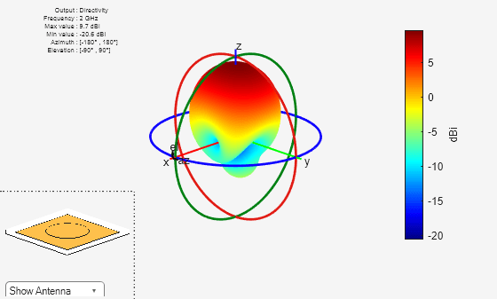

Create the two element linear array antenna using the patchMicrostripCircular object and use it in the Antenna block as receiver antenna. Visualize the antenna using the show command. Any other antenna can also be used as a receiver like a spiral or a dipole blade.

ant = design(patchMicrostripCircular,2.5e9);
antRx = linearArray(NumElements = 2,Element = ant);
antRx.ElementSpacing = lambda/2;
figure
show(antRx);
title("Linear Array of Circular Patch Antennas")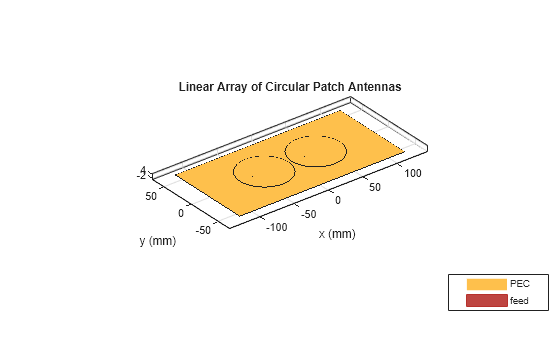

Calculate the pattern using the pattern function.

figure
pattern(antRx,2e9);

After adding the transmit and receive antenna in the Antenna block, visualize the model using the open_system command.

The model consists of a transmitter and a receiver, and the receiver section has two channels which are fed by a two-element linear array. The phase difference between the channels are calculated and the angle of arrival is estimated. The phase from each antenna needs to be calibrated to generate an accurate phase difference and hence the Phase Shifter blocks are connected to both the RF Channels.

Phase shifter block measures the phase shift of both the antennas when the emitter location is in boresight and using a phase shift to cancel that phase to make it 0 deg for the receive angle. This ensures that when the emitter is directed towards the left of boresight the resultant phase difference is negative and its positive when the emitter is directed towards the right of boresight as shown in the phase plot below.

open_system('PhaseComparisonTechnique_1.slx');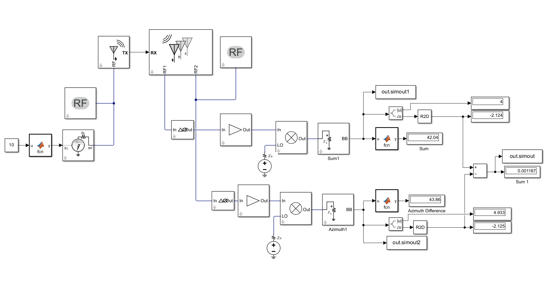

Simulate the model and calculate the angle of arrival. This angle must be close to the previously initialized emitter location. The coordinate system in the Antenna Toolbox is slightly different than the conventional spherical coordinate system. The elevation angle starts at x=0 as compared to z=0 in the conventional spherical coordinate system. Hence add 90 degrees to the input emitter location to correctly specify its value. Place the antenna normal to the z-axis so that it detects the target in the -90 to +90 elevation range.

emitterLocation = -30; % Value between -90 to 90 for Source Location
d = antRx.ElementSpacing;
thetaEmitter = emitterLocation + 90; 
out1= sim('PhaseComparisonTechnique_1.slx',0);
PhaseDifference = out1.simout.Data;
AoA = rad2deg(asin((c*PhaseDifference*(pi/180))/(2*pi*freq*d)))

AoA = 
-32.6581

This code generates a phase difference at every angle of arrival defined by the theta variable. The plot changes based on the spacing between the antennas. Run this code at your command line to calculate the phase difference at various theta values for this antenna array.

theta = 0:5:180;
for i=1:numel(theta)
thetaEmitter = theta(i);
out1= sim('PhaseComparisonTechnique_1.slx',0);
out2(i) = out1.simout.Data;
end
figure,plot(theta,out2);
grid on
title("Phase Difference value for different Angle of Arrival");
xlabel("Angle of Arrival");
ylabel("Phase Difference");

Antenna Array Modeled Using Measured Data

The second way to compute AoA is by using the measuredAntenna object. Here we model the antenna array using measured data. Use the embedded element EH near field data and the antenna S-parameters. You can use the data from measurements or from a third party EM analysis tools. In this example, data obtained from a full-wave analysis in Antenna Toolbox is used.

Compute the embedded and total electric fields for the receive antenna array using the EHfields function. Assign this data to the measuredAntenna object, and then use this antenna within the model to calculate the Angle of Arrival (AoA).

az = -180:5:180;
el = -90:5:90;
R = 14.5;
ant = antRx;
phi1 = az;
theta1 = 90-el;
coord = 'polar';
% [Points,phi,theta] = em.internal.calcpointsinspace( phi1, theta1, R,coord);
[theta,phi] = meshgrid(theta1,phi1);
[mp,np] = size(phi);
[mt,nt] = size(theta);
phi = phi(:);
theta = theta(:);
x = R.*sind(theta).*cosd(phi);
y = R.*sind(theta).*sind(phi);
z = R.*cosd(theta);
Points = [x';y';z'];
phi = reshape(phi,mp,np);
theta = reshape(theta,mt,nt);

Etotal = zeros(size(Points,2),3,numel(freq));
EmbE = zeros(size(Points,2),3,ant.NumElements,numel(freq));
for n = 1:numel(freq)
    E0 = EHfields(ant,freq(n),Points);
    Etotal(:,:,n) = E0.';
    for m = 1:ant.NumElements
        E1 = EHfields(ant,freq(n),Points,ElementNumber = m,Termination = 46);
        EmbE(:,:,m,n) = E1.';
    end
end
Dir = [phi(:) 90-theta(:) R*ones(numel(phi),1)];
sparamVal = sparameters(ant,freq);
mesAnt = measuredAntenna(E=abs(E0.'),Direction=Dir,NumPorts=2,...
                Azimuth=az,Elevation=90-el,FieldCoordinate='rectangular',...
                EmbeddedE=EmbE,FieldFrequency=freq,Sparameters=sparamVal,PhaseCenter=[0 0 0]);
antRx = mesAnt;

Simulate the model and calculate the angle of arrival which must match with the emitter location

out1= sim('PhaseComparisonTechnique_1.slx',0);
PhaseDifference = out1.simout.Data;
AoAwithMeasured = rad2deg(asin((c*PhaseDifference*(pi/180))/(2*pi*freq*d)))

AoAwithMeasured = 
-32.6964

The simulation model for estimating the angle of arrival (AoA) accurately aligns with the emitter location in both scenarios, underscoring its precision in determining signal direction. By integrating real-world measurement data, the model can directly compute the AoA, enhancing its practical utility. This method not only confirms the system's functionality but also evaluates its performance under various impairments, ensuring that the AoA is detected within acceptable limits. As a result, the model acts as a reliable tool for verifying system accuracy and dependability in environments prone to signal interference or distortion, making it invaluable for applications such as radar, sonar, and wireless communications.

Conclusion

The model-based design approach highlighted in this example offers a valuable framework for simulating and optimizing direction-finding systems through phase comparison techniques. The results from both approaches closely match the emitter location used. By integrating antenna and RF components into a unified model, designers can predict performance and make informed decisions regarding system design and implementation. This method improves the efficiency of development and testing processes, ultimately leading to more effective direction-finding solutions.

References

[1] Sourabh Joshi, Shashank Kulkarni, and Giorgia Zucchelli. "Model-Based Design for Direction Finding with Phase Comparison." In 2024 IEEE International Symposium on Antennas and Propagation and INC/USNC‐URSI Radio Science Meeting (AP-S/INC-USNC-URSI), 2117–18. Firenze, Italy: IEEE, 2024. https://doi.org/10.1109/AP-S/INC-USNC-URSI52054.2024.10686668.