Estimate Angle of Arrival Using Amplitude Comparison

Since R2025a

This example shows how to estimate the angle of arrival using the amplitude comparison technique.

In this approach, an antenna array scans the area of interest, and then the location of the emitter is estimated based on the maximum received signal power. A circular patch antenna serves as a transmitter antenna, while a 16-element blade dipole array functions as a receiver antenna. The transmitter is included to demonstrate the completeness of the model and to show that such systems can also be constructed. The estimation of the angle of arrival is implemented at the receiver.

Transmit and Receive Antenna

Use the patchMicrostripCircular object to design a 4-element linear array for the transmitter antenna. Use the pattern function to visualize the antenna pattern.

fc = 2e9;
warning off;
ant = patchMicrostripCircular;
ant = design(ant,fc);
arrayTX_AC = design(linearArray(NumElements = 4),fc,ant);
figure
pattern(arrayTX_AC,fc);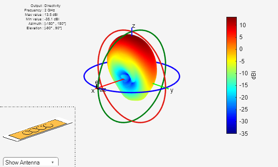

Use the reflector and dipoleBlade objects to create the rectangular array of 16 elements. The receiver antenna is a 16-element blade dipole rectangular array.

ant = reflector;
ex = design(dipoleBlade,fc);
ant = design(ant,fc);
ant.Exciter = ex;
ant.Exciter.Tilt = 90;
ant.Exciter.TiltAxis = [0 1 0];
arrayRX_AC = rectangularArray(Size = [4 4]);
arrayRX_AC = design(arrayRX_AC,fc,ant);

Visualize the array using the show function.

figure
show(arrayRX_AC);
title('Rectangular Array of Reflectors');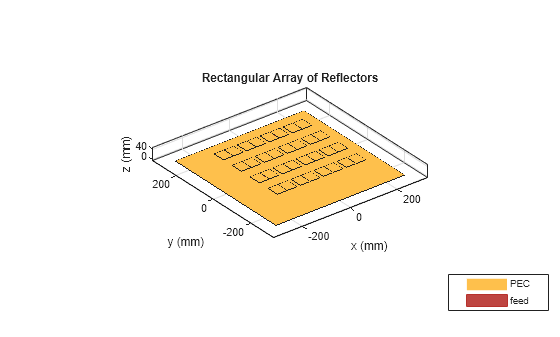

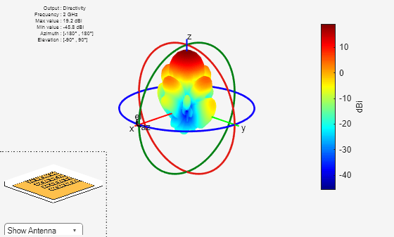
Calculate the radiation pattern of the array using the pattern function. The gain of the array is 19.2 dBi and the pattern is symmetrical in both the E and H planes.

figure
pattern(arrayRX_AC,fc);

Configure a 4-by-4 uniform rectangular antenna array (URA) with elements spaced according to specified row and column spacing, oriented along the Z-axis. Calculate the effective diameter of the array by determining the distance between specific elements. Minimize the side lobe level by applying a Taylor taper. This taper values are used in the amplifier design to reduce the SLL.

nbar = 2;
sll = -25;
arr = phased.URA;
arr.Size = [4 4];
arr.ArrayNormal = 'z';
arr.ElementSpacing = [arrayRX_AC.RowSpacing arrayRX_AC.ColumnSpacing];
pos = getElementPosition(arr);
diff = pos(:,13)-pos(:,4);
diff = diff.^2;
sum1 = sum(diff);
diam = sqrt(sum1);
Taper = taylortaperc(pos,diam,nbar,sll);
tay = 20*log10(Taper);

Receiver Model

The receiver is modeled in RF Blockset™ Circuit Envelope simulation environment to refine transceiver architectures with increased modeling fidelity. The receive section incorporates a beamforming network with variable phase shifters linked to each antenna element. The 16 outputs are combined using power combiner blocks and then downconverted to baseband.

The antenna beam scans the area of interest, measuring power at each scan. The angle at which maximum power is received indicates the direction of the emitter. Amplifiers are connected to the receiver antenna array to utilize Taylor series coefficients, effectively reducing the side lobe level (SLL). This approach ensures more accurate determination of the emitter's location by minimizing interference from side lobes during the beam scanning process.

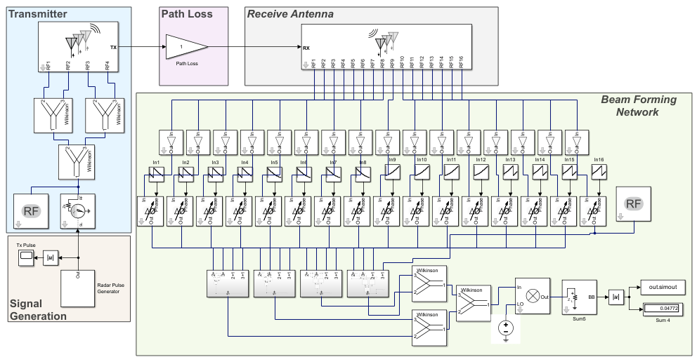
open_system('amplitudeComparisonAoA.slx');

Simulation and Results

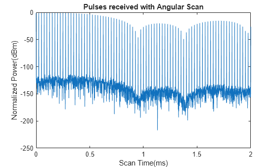
Run the below code to simulate an angular scan to estimate the angle of arrival using the amplitude comparison. Set the search area from -40 to +40 degrees in the elevation plane, with thetaEmitter at -30 degrees. For each angle, the model calculates the phase shift for scanning the beam. Run the model using the sim function to simulate the scan over the defined step time. Plot the output from the model which shows the received pulses during the angular scan.

thetaEmitter = -30; % -40 deg to +40 deg is the search area
Step_Time = 0.025;
angleAz = 50:1:130;
angleInput = thetaEmitter + 90; 
for i=1:numel(angleAz)
ps1(:,i) = phaseShift(arrayRX_AC,2e9,[0;angleAz(i)]);
end
ps = ps1';
out = sim('amplitudeComparisonAoA.slx',(Step_Time*(numel(angleAz)-1)));
figure
plot(out.simout.Time,20*log10(abs(out.simout.Data)))
title("Pulses received with Angular Scan");
xlabel("Scan Time(ms)");
ylabel("Normalized Power(dBm)");

Estimate the value of AoA by processing the data received from the model. The estimated value closely matches the direction of the emitter.

Dataout = 20*log10(abs(out.simout.Data));
thresh = mean(Dataout);
Noise = Dataout(Dataout<mean(Dataout));
Sig = Dataout(Dataout>-60);
[val,id1]=max(Sig);
DirectionEmitter = angleAz(id1) - 90

DirectionEmitter = 
-33

The emitter location is estimated correctly with the estimated value close to the actual emitter location which shows the system is performing as expected. This example can be expanded to perform scanning in both azimuth and elevation, allowing for the determination of the emitter's location in 3-D space. Additionally, increasing the number of elements in the receive antenna can help achieve a narrower beam.

References

[1] Joshi, Sourabh Mukund, and Shashank Kulkarni. "Model-Based Design for Direction-Finding with Amplitude Comparison". IEEE Wireless Antenna and Microwave Symposium (WAMS), 1–4. Visakhapatnam, India: IEEE, 2024. https://doi.org/10.1109/WAMS59642.2024.10528021