Fit One-Compartment Model to Individual PK Profile
Background
This example shows how to fit an individual's PK profile data to one-compartment model and estimate pharmacokinetic parameters.
Suppose you have drug plasma concentration data from an individual and want to estimate the volume of the central compartment and the clearance. Assume the drug concentration versus the time profile follows the monoexponential decline , where is the drug concentration at time t, is the initial concentration, and is the elimination rate constant that depends on the clearance and volume of the central compartment .
The synthetic data in this example was generated using the following model, parameters, and dose:
One-compartment model with bolus dosing and first-order elimination
Volume of the central compartment (
Central) = 1.70 literClearance parameter (
Cl_Central) = 0.55 liter/hourConstant error model
Bolus dose of 10 mg
Load Data and Visualize
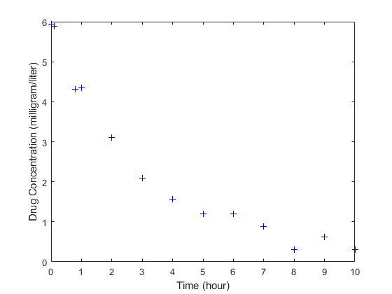
The data is stored as a table with variables Time and Conc that represent the time course of the plasma concentration of an individual after an intravenous bolus administration measured at 13 different time points. The variable units for Time and Conc are hour and milligram/liter, respectively.
load('data15.mat')
plot(data.Time,data.Conc,'b+')
xlabel('Time (hour)');
ylabel('Drug Concentration (milligram/liter)');
Convert to groupedData Format
Convert the data set to a groupedData object, which is the required data format for the fitting function sbiofit for later use. A groupedData object also lets you set independent variable and group variable names (if they exist). Set the units of the Time and Conc variables. The units are optional and only required for the UnitConversion feature, which automatically converts matching physical quantities to one consistent unit system.
gData = groupedData(data);
gData.Properties.VariableUnits = {'hour','milligram/liter'};
gData.Properties
ans = struct with fields:
Description: ''
UserData: []
DimensionNames: {'Row' 'Variables'}
VariableNames: {'Time' 'Conc'}
VariableDescriptions: {}
VariableUnits: {'hour' 'milligram/liter'}
VariableContinuity: []
RowNames: {}
CustomProperties: [1×1 matlab.tabular.CustomProperties]
GroupVariableName: ''
IndependentVariableName: 'Time'
groupedData automatically set the name of the IndependentVariableName property to the Time variable of the data.
Construct a One-Compartment Model
Use the built-in PK library to construct a one-compartment model with bolus dosing and first-order elimination where the elimination rate depends on the clearance and volume of the central compartment. Use the configset object to turn on unit conversion.
pkmd                    = PKModelDesign;
pkc1                    = addCompartment(pkmd,'Central');
pkc1.DosingType         = 'Bolus';
pkc1.EliminationType    = 'linear-clearance';
pkc1.HasResponseVariable = true;
model                   = construct(pkmd);
configset               = getconfigset(model);
configset.CompileOptions.UnitConversion = true;
For details on creating compartmental PK models using the SimBiology® built-in library, see Create Pharmacokinetic Models.
Define Dosing
Define a single bolus dose of 10 milligram given at time = 0. For details on setting up different dosing schedules, see Doses in SimBiology Models.
dose                = sbiodose('dose');
dose.TargetName     = 'Drug_Central';
dose.StartTime      = 0;
dose.Amount         = 10;
dose.AmountUnits    = 'milligram';
dose.TimeUnits      = 'hour';
Map Response Data to the Corresponding Model Component
The data contains drug concentration data stored in the Conc variable. This data corresponds to the Drug_Central species in the model. Therefore, map the data to Drug_Central as follows.
responseMap = {'Drug_Central = Conc'};Specify Parameters to Estimate
The parameters to fit in this model are the volume of the central compartment (Central) and the clearance rate (Cl_Central). In this case, specify log-transformation for these biological parameters since they are constrained to be positive. The estimatedInfo object lets you specify parameter transforms, initial values, and parameter bounds if needed.
paramsToEstimate    = {'log(Central)','log(Cl_Central)'};
estimatedParams     = estimatedInfo(paramsToEstimate,'InitialValue',[1 1],'Bounds',[1 5;0.5 2]);
Estimate Parameters
Now that you have defined one-compartment model, data to fit, mapped response data, parameters to estimate, and dosing, use sbiofit to estimate parameters. The default estimation function that sbiofit uses will change depending on which toolboxes are available. To see which function was used during fitting, check the EstimationFunction property of the corresponding results object.
fitConst = sbiofit(model,gData,responseMap,estimatedParams,dose);
Display Estimated Parameters and Plot Results
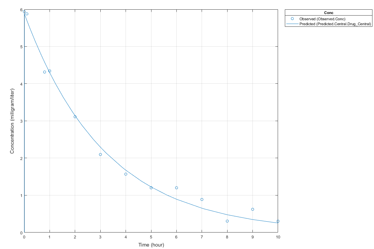
Notice the parameter estimates were not far off from the true values (1.70 and 0.55) that were used to generate the data. You may also try different error models to see if they could further improve the parameter estimates.
fitConst.ParameterEstimates
ans=2×4 table
         Name         Estimate    StandardError      Bounds
    ______________    ________    _____________    __________

    {'Central'   }     1.6993       0.034821         1      5
    {'Cl_Central'}    0.53358        0.01968       0.5      2
s.Labels.XLabel     = 'Time (hour)';
s.Labels.YLabel     = 'Concentration (milligram/liter)';
plot(fitConst,'AxesStyle',s);
Use Different Error Models
Try three other supported error models (proportional, combination of constant and proportional error models, and exponential).
fitProp = sbiofit(model,gData,responseMap,estimatedParams,dose,...
                      'ErrorModel','proportional');
fitExp  = sbiofit(model,gData,responseMap,estimatedParams,dose,...
                      'ErrorModel','exponential');
fitComb = sbiofit(model,gData,responseMap,estimatedParams,dose,...
                      'ErrorModel','combined');
Use Weights Instead of an Error Model
You can specify weights as a numeric matrix, where the number of columns corresponds to the number of responses. Setting all weights to 1 is equivalent to the constant error model.
weightsNumeric = ones(size(gData.Conc));
fitWeightsNumeric = sbiofit(model,gData,responseMap,estimatedParams,dose,'Weights',weightsNumeric);
Alternatively, you can use a function handle that accepts a vector of predicted response values and returns a vector of weights. In this example, use a function handle that is equivalent to the proportional error model.
weightsFunction = @(y) 1./y.^2;
fitWeightsFunction = sbiofit(model,gData,responseMap,estimatedParams,dose,'Weights',weightsFunction);
Compare Information Criteria for Model Selection
Compare the loglikelihood, AIC, and BIC values of each model to see which error model best fits the data. A larger likelihood value indicates the corresponding model fits the model better. For AIC and BIC, the smaller values are better.
allResults = [fitConst,fitWeightsNumeric,fitWeightsFunction,fitProp,fitExp,fitComb];
errorModelNames = {'constant error model','equal weights','proportional weights', ...
                   'proportional error model','exponential error model',...
                   'combined error model'};
LogLikelihood = [allResults.LogLikelihood]';
AIC = [allResults.AIC]';
BIC = [allResults.BIC]';
t = table(LogLikelihood,AIC,BIC);
t.Properties.RowNames = errorModelNames;
tt=6×3 table
LogLikelihood AIC BIC
_____________ _______ _______
constant error model 3.9866 -3.9732 -2.8433
equal weights 3.9866 -3.9732 -2.8433
proportional weights -3.8472 11.694 12.824
proportional error model -3.8257 11.651 12.781
exponential error model 1.1984 1.6032 2.7331
combined error model 3.9163 -3.8326 -2.7027
Based on the information criteria, the constant error model (or equal weights) fits the data best since it has the largest loglikelihood value and the smallest AIC and BIC.
Display Estimated Parameter Values
Show the estimated parameter values of each model.
Estimated_Central       = zeros(6,1);
Estimated_Cl_Central    = zeros(6,1);
t2 = table(Estimated_Central,Estimated_Cl_Central);
t2.Properties.RowNames = errorModelNames;
for i = 1:height(t2)
    t2{i,1} = allResults(i).ParameterEstimates.Estimate(1);
    t2{i,2} = allResults(i).ParameterEstimates.Estimate(2);
end
t2
t2=6×2 table
                                Estimated_Central    Estimated_Cl_Central
                                _________________    ____________________

    constant error model             1.6993                0.53358
    equal weights                    1.6993                0.53358
    proportional weights             1.9045                0.51734
    proportional error model         1.8777                0.51147
    exponential error model          1.7872                0.51701
    combined error model             1.7008                0.53271
Conclusion
This example showed how to estimate PK parameters, namely the volume of the central compartment and clearance parameter of an individual, by fitting the PK profile data to one-compartment model. You compared the information criteria of each model and estimated parameter values of different error models to see which model best explained the data. Final fitted results suggested both the constant and combined error models provided the closest estimates to the parameter values used to generate the data. However, the constant error model is a better model as indicated by the loglikelihood, AIC, and BIC information criteria.
See Also
Related Topics
Select a Web Site
Choose a web site to get translated content where available and see local events and offers. Based on your location, we recommend that you select: United States.
You can also select a web site from the following list
Americas
- América Latina (Español)
- Canada (English)
- United States (English)
Europe
- Belgium (English)
- Denmark (English)
- Deutschland (Deutsch)
- España (Español)
- Finland (English)
- France (Français)
- Ireland (English)
- Italia (Italiano)
- Luxembourg (English)
- Netherlands (English)
- Norway (English)
- Österreich (Deutsch)
- Portugal (English)
- Sweden (English)
- Switzerland
- United Kingdom (English)
Asia Pacific
- Australia (English)
- India (English)
- New Zealand (English)
- 中国
- 日本Japanese (日本語)
- 한국Korean (한국어)