Reconstruct Missing Data
This example shows how to reconstruct missing data via interpolation, anti-aliasing filtering, and autoregressive modeling.
Introduction
With the advent of cheap data acquisition hardware, you often have access to signals that are rapidly sampled at regular intervals. This allows you to gain a fine approximation to the underlying signal. But what happens when the data you are measuring are coarsely sampled or otherwise missing significant portions? How do you infer the values of the signals at points in between the samples that you know?
Linear Interpolation
Linear interpolation is by far the most common method of inferring values between sampled points. By default, when you plot a vector in MATLAB®, you see the points connected by straight lines. You need to sample a signal at very fine detail in order to approximate the true signal.
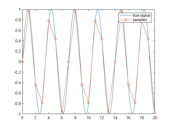
In this example, a sinusoid is sampled with both fine and coarse resolution. When plotted on a graph, the finely sampled sinusoid very closely resembles what the true continuous sinusoid would look like. Thus, you can use it as a model of the "true signal." In the plot below, the samples of a coarsely sampled signal are shown as circles connected by straight lines.
tTrueSignal = 0:0.01:20;
xTrueSignal = sin(2*pi*2*tTrueSignal/7);

tSampled = 0:20;
xSampled = sin(2*pi*2*tSampled/7);

plot(tTrueSignal,xTrueSignal,"-",tSampled,xSampled,"o-")
legend("true signal","samples")
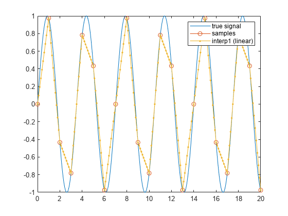
It is straightforward to recover intermediate samples in the same way that plot performs interpolation. This can be accomplished with the linear method of the interp1 function.
tResampled = 0:0.1:20;
xLinear = interp1(tSampled,xSampled,tResampled,"linear");
plot(tTrueSignal,xTrueSignal,"-", ...
     tSampled, xSampled, "o-", ...
     tResampled,xLinear,".-")
legend("true signal","samples","interp1 (linear)")
The problem with linear interpolation is that the result is not very smooth. Other interpolation methods can produce smoother approximations.
Spline Interpolation
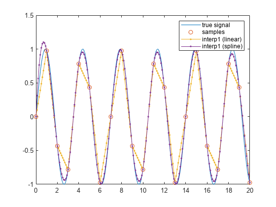
Many physical signals are like sinusoids in that they are continuous and have continuous derivatives. You can reconstruct such signals by using cubic spline interpolation, which ensures that the first and second derivatives of the interpolated signal are continuous at every data point:
xSpline = interp1(tSampled,xSampled,tResampled,"spline");
plot(tTrueSignal,xTrueSignal,"-", ...
     tSampled, xSampled,"o", ...
     tResampled,xLinear,".-", ...
     tResampled,xSpline,".-")
legend("true signal","samples","interp1 (linear)","interp1 (spline)")
Cubic splines are particularly effective when interpolating signals that consist of sinusoids. However, there are other techniques that can be used to gain greater fidelity to physical signals which have continuous derivatives up to a very high order.
Resampling with Antialiasing Filters
The resample function in the Signal Processing Toolbox provides another technique to fill in missing data. resample can reconstruct sinusoidal components of low frequency with very low distortion.
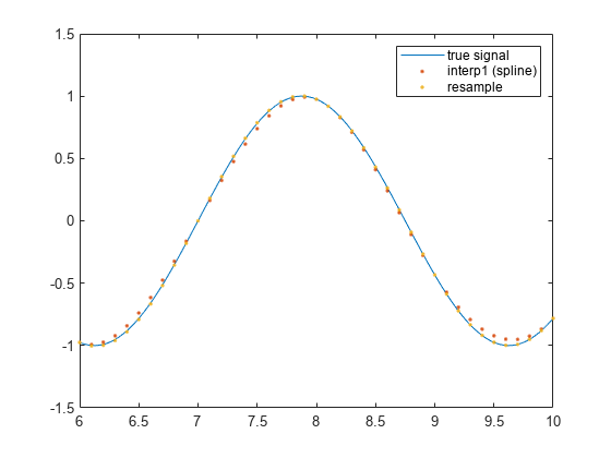
xResample = resample(xSampled, 10, 1);
tResample = 0.1*((1:numel(xResample))-1);

plot(tTrueSignal,xTrueSignal,"-", ...
     tResampled,xSpline,".", ...
     tResample, xResample,".")
legend("true signal","interp1 (spline)","resample")
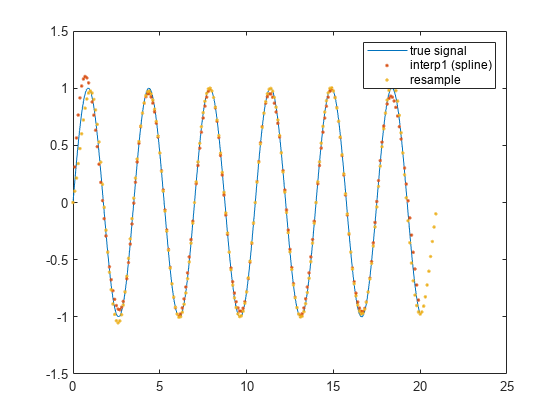
Like the other methods, resample has some difficulty reconstructing the endpoints. On the other hand, the central portion of the reconstructed signal agrees very well with the true signal.
xlim([6 10])
Resampling with Missing Samples
resample can accommodate nonuniformly sampled signals. The technique works best when the signal is sampled at a high rate.
In the following example, we create a slowly moving sinusoid, remove a sample, and zoom into the vicinity of the missing sample.
tTrueSignal = 0:.1:20;
xTrueSignal = sin(2*pi*2*tTrueSignal/15);

Tx = 0:20;

Tmissing = Tx(10);
Tx(10) = [];

x = sin(2*pi*2*Tx/15);
Xmissing = sin(2*pi*2*Tmissing/15);

[y, Ty] = resample(x,Tx,10,"spline");

plot(tTrueSignal, xTrueSignal, "-", ...
     Tmissing,Xmissing,"x ", ...
     Tx,x,"o ", ...
     Ty,y,". ")
legend("true signal","missing sample", ...
    "remaining samples","resample with ""spline""")
ylim([-1.2 1.2])
xlim([6 14])
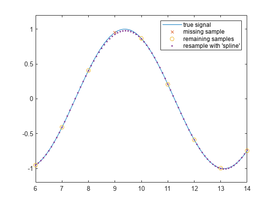
The reconstructed sinusoid tracks the shape of the true signal reasonably well, with only a slight error in the vicinity of the missing sample.
However, resample does not work well when there is a large gap in the signal. For example, consider a dampened sinusoid whose middle portion is missing:
tTrueSignal = (0:199)/199;
xTrueSignal = exp(-0.5*tTrueSignal).*sin(2*pi*5*tTrueSignal);

tMissing = tTrueSignal;
xMissing = xTrueSignal;
tMissing(50:140) = [];
xMissing(50:140) = [];

[y,Ty] = resample(xMissing, tMissing, 200, "spline");

plot(tTrueSignal,xTrueSignal,"-", ...
     tMissing,xMissing,"o",...
     Ty,y,".")
legend("true signal","samples","resample with ""spline""")
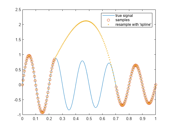
Here resample ensures that the reconstructed signal is continuous and has continuous derivatives in the vicinity of the missing points. However, it cannot adequately reconstruct the missing portion.
Reconstructing Large Gaps
As can be seen above, filtering and cubic interpolation alone might not be sufficient to deal with large gaps. However, with certain kinds of sampled signals, such as those that arise when observing oscillating phenomena, you can often infer the values of missing samples based upon the data immediately preceding or following the gap.
The fillgaps function can replace missing samples (specified by NaN) in an otherwise uniformly sampled signal by fitting an autoregressive model to the samples surrounding a gap and extrapolating into the gap from both directions.
tTrueSignal = (0:199)/199;
xTrueSignal = exp(-.5*tTrueSignal).*sin(2*pi*5*tTrueSignal);
gapSignal = xTrueSignal;
gapSignal(50:140) = NaN;
y = fillgaps(gapSignal);

plot(tTrueSignal,xTrueSignal,"-", ...
     tTrueSignal,gapSignal,"o", ...
     tTrueSignal,y,".")

legend("true signal","samples","reconstructed signal")
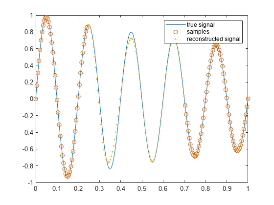
The technique works because autoregressive signals have information that is spread out over many samples. Only a few samples within any segment are needed to completely reconstruct the full signal.
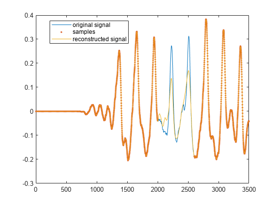
This type of reconstruction can be adapted to estimate missing samples of more complicated signals. Consider a sampled audio signal of a plucked guitar string after removing six hundred samples immediately after the pluck:
[y,fs] = audioread("guitartune.wav");
x = y(1:3500);
x(2000:2600) = NaN;
y2 = fillgaps(x);
plot(1:3500, y(1:3500), "-", ...
     1:3500, x, ".", ...
     1:3500, y2, "-")
legend("original signal","samples","reconstructed signal",...
       Location="best")
Reconstructing Gaps with Localized Estimation
It is fairly straightforward to fill data within a gap when it is known that the signal in the vicinity of the gap can be modeled with a single autoregressive process. You can mitigate problems when a signal consists of a non-constant autoregressive process by restricting the area over which the model parameters are computed. This is useful when you are trying to fill a gap within the "ringing" period of one resonance that comes immediately before or after another, stronger, resonance.
x = y(350001:370000);
x(6000:6950) = NaN;
y2 = fillgaps(x);
y3 = fillgaps(x,1500);
plot(1:20000, y(350001:370000), "-", ...
     1:20000, x, ".", ...
     1:20000, y2, "-", ...
     1:20000, y3, "-")
xlim([2200 10200])
legend("original signal","samples", ...
    "fillgaps (all)","fillgaps (localized)",Location="best")
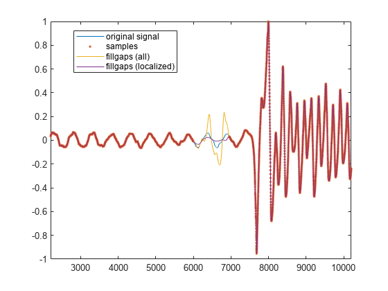
In the plot above, the waveform is missing a section just before a large resonance. As before, fillgaps is used to extrapolate into the gap region using all available data. A second call to fillgaps uses only 1500 samples on either side of the gap to perform the modeling. This mitigates the effect of the subsequent guitar pluck after sample 7500.
Summary
You have seen several ways to reconstruct missing data from its neighboring sample values using interpolation, resampling and autoregressive modeling.
Interpolation and resampling work for slowly varying signals. Resampling with antialiasing filters often does a better job at reconstructing signals that consist of low-frequency components. For reconstructing large gaps in oscillating signals, autoregressive modeling in the vicinity of the gap can be particularly effective.