Signal Generation and Visualization
This example shows how to generate widely used periodic and aperiodic waveforms, swept-frequency sinusoids, and pulse trains using functions available in Signal Processing Toolbox™.
Periodic Waveforms
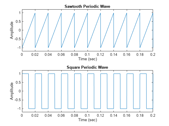
In addition to the sin and cos functions in MATLAB®, Signal Processing Toolbox™ offers other functions, such as sawtooth and square, that produce periodic signals.
The sawtooth function generates a sawtooth wave with peaks at and a period of . An optional width parameter specifies a fractional multiple of at which the signal's maximum occurs.
The square function generates a square wave with a period of . An optional parameter specifies duty cycle, the percent of the period for which the signal is positive.
Generate 1.5 seconds of a 50 Hz sawtooth wave with a sample rate of 10 kHz. Repeat the computation for a square wave.
fs = 10000;
t = 0:1/fs:1.5;
x1 = sawtooth(2*pi*50*t);
x2 = square(2*pi*50*t);

nexttile
plot(t,x1)
axis([0 0.2 -1.2 1.2])
xlabel("Time (sec)")
ylabel("Amplitude")
title("Sawtooth Periodic Wave")

nexttile
plot(t,x2)
axis([0 0.2 -1.2 1.2])
xlabel("Time (sec)")
ylabel("Amplitude")
title("Square Periodic Wave")
Aperiodic Waveforms
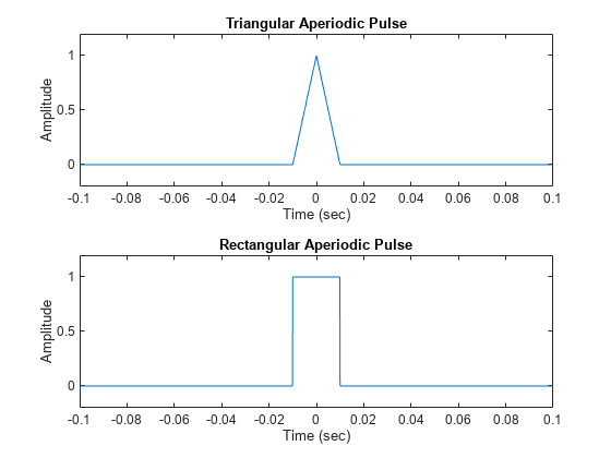
To generate triangular, rectangular and Gaussian pulses, the toolbox offers the tripuls, rectpuls, and gauspuls functions.
The tripuls function generates a sampled aperiodic, unit-height triangular pulse centered about t = 0 and with a default width of 1.
The rectpuls function generates a sampled aperiodic, unit-height rectangular pulse centered about t = 0 and with a default width of 1. The interval of nonzero amplitude is defined to be open on the right: rectpuls(-0.5) = 1 while rectpuls(0.5) = 0.
Generate 2 seconds of a triangular pulse with a sample rate of 10 kHz and a width of 20 ms. Repeat the computation for a rectangular pulse.
fs = 10000;
t = -1:1/fs:1;
x1 = tripuls(t,20e-3);
x2 = rectpuls(t,20e-3);

figure
nexttile
plot(t,x1)
axis([-0.1 0.1 -0.2 1.2])
xlabel("Time (sec)")
ylabel("Amplitude")
title("Triangular Aperiodic Pulse")

nexttile
plot(t,x2)
axis([-0.1 0.1 -0.2 1.2])
xlabel("Time (sec)")
ylabel("Amplitude")
title("Rectangular Aperiodic Pulse")
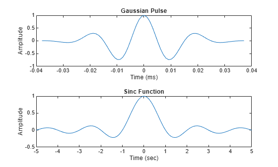
The gauspuls function generates a Gaussian-modulated sinusoidal pulse with a specified time, center frequency, and fractional bandwidth.
The sinc function computes the mathematical sinc function for an input vector or matrix. The sinc function is the continuous inverse Fourier transform of a rectangular pulse of width and unit height.
Generate a 50 kHz Gaussian RF pulse with 60% bandwidth, sampled at a rate of 1 MHz. Truncate the pulse where the envelope falls 40 dB below the peak.
tc = gauspuls("cutoff",50e3,0.6,[],-40);
t1 = -tc : 1e-6 : tc;
y1 = gauspuls(t1,50e3,0.6);
Generate the sinc function for a linearly spaced vector:
t2 = linspace(-5,5);
y2 = sinc(t2);

figure
nexttile
plot(t1*1e3,y1)
xlabel("Time (ms)")
ylabel("Amplitude")
title("Gaussian Pulse")

nexttile
plot(t2,y2)
xlabel("Time (sec)")
ylabel("Amplitude")
title("Sinc Function")
Swept-Frequency Waveforms
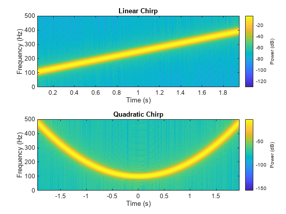
The toolbox also provides functions to generate swept-frequency waveforms such as the chirp function. Two optional parameters specify alternative sweep methods and initial phase in degrees. Below are several examples of using the chirp function to generate linear or quadratic, convex, and concave quadratic chirps.
Generate a linear chirp sampled at 1 kHz for 2 seconds. The instantaneous frequency is 100 Hz at t = 0 and crosses 250 Hz at t = 1 second.
tlin = 0:0.001:2;
ylin = chirp(tlin,100,1,250);
Generate a quadratic chirp sampled at 1 kHz for 4 seconds. The instantaneous frequency is 100 Hz at t = 0 and crosses 200 Hz at t = 1 second.
tq = -2:0.001:2;
yq = chirp(tq,100,1,200,"quadratic");
Compute and display the spectrograms of the chirps.
figure
nexttile
pspectrum(ylin,tlin,"spectrogram", ...
    Leakage=0.85,TimeResolution=0.1,OverlapPercent=99)
title("Linear Chirp")

nexttile
pspectrum(yq,tq,"spectrogram", ...
    Leakage=0.85,TimeResolution=0.1,OverlapPercent=99)
title("Quadratic Chirp")
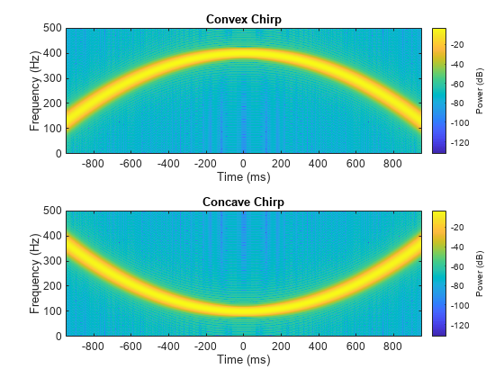
Generate a convex quadratic chirp sampled at 1 kHz for 2 seconds. The instantaneous frequency is 100 Hz at t = 0 and increases to 400 Hz at t = 1 second.
tcx = -1:0.001:1;
fo = 100;
f1 = 400;
ycx = chirp(tcx,fo,1,f1,"quadratic",[],"convex");
Generate a concave quadratic chirp sampled at 1 kHz for 2 seconds. The instantaneous frequency is 400 Hz at t = 0 and decreases to 100 Hz at t = 1 second.
tcv = -1:0.001:1;
fo = 400;
f1 = 100;
ycv = chirp(tcv,fo,1,f1,"quadratic",[],"concave");
Compute and display the spectrograms of the chirps.
figure
nexttile
pspectrum(ycx,tcx,"spectrogram", ...
    Leakage=0.85,TimeResolution=0.1,OverlapPercent=99)
title("Convex Chirp")

nexttile
pspectrum(ycv,tcv,"spectrogram", ...
    Leakage=0.85,TimeResolution=0.1,OverlapPercent=99)
title("Concave Chirp")
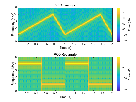
Another function generator is the vco (voltage-controlled oscillator), which generates a signal oscillating at a frequency determined by the input vector. The input vector can be a triangle, a rectangle, or a sinusoid, among other possibilities.
Generate 2 seconds of a signal sampled at 10 kHz whose instantaneous frequency is a triangle. Repeat the computation for a rectangle.
fs = 10000;
t = 0:1/fs:2;
x1 = vco(sawtooth(2*pi*t,0.75),[0.1 0.4]*fs,fs);
x2 = vco(square(2*pi*t),[0.1 0.4]*fs,fs);
Plot the spectrograms of the generated signals.
figure
nexttile
pspectrum(x1,t,"spectrogram", ...
    Leakage=0.9,FrequencyResolution=55)
title("VCO Triangle")

nexttile
pspectrum(x2,t,"spectrogram", ...
    Leakage=0.9,FrequencyResolution=55)
title("VCO Rectangle")
Pulse Trains
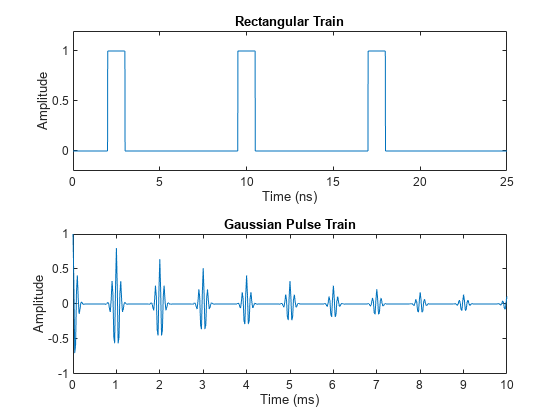
To generate pulse trains, you can use the pulstran function.
Construct a train of 1 ns rectangular pulses sampled at a rate of 100 GHz with a spacing of 7.5 ns.
fs = 100e9;
D = [2.5 10 17.5]' * 1e-9;
t = 0 : 1/fs : 2500/fs;
w = 1e-9;
yp = pulstran(t,D,@rectpuls,w);
Generate a periodic Gaussian pulse signal at 10 kHz with 50% bandwidth. The pulse repetition frequency is 1 kHz, the sample rate is 50 kHz, and the pulse train length is 10 milliseconds. The repetition amplitude should attenuate by 0.8 each time. Uses a function handle to specify the generator function.
T = 0 : 1/50e3 : 10e-3;
D = [0 : 1/1e3 : 10e-3 ; 0.8.^(0:10)]';
Y = pulstran(T,D,@gauspuls,10e3,.5);

figure
nexttile
plot(t*1e9,yp)
axis([0 25 -0.2 1.2])
xlabel("Time (ns)")
ylabel("Amplitude")
title("Rectangular Train")

nexttile
plot(T*1e3,Y)
xlabel("Time (ms)")
ylabel("Amplitude")
title("Gaussian Pulse Train")
See Also
chirp | gauspuls | pulstran | rectpuls | sawtooth | sin | sinc | square | tripuls | vco
You can also select a web site from the following list:
Americas
- América Latina (Español)
- Canada (English)
- United States (English)
Europe
- Belgium (English)
- Denmark (English)
- Deutschland (Deutsch)
- España (Español)
- Finland (English)
- France (Français)
- Ireland (English)
- Italia (Italiano)
- Luxembourg (English)
- Netherlands (English)
- Norway (English)
- Österreich (Deutsch)
- Portugal (English)
- Sweden (English)
- Switzerland
- United Kingdom (English)